David Schmidt, Kansas State University, USA
How do we design and calculate the behavior of a computer program before building it? This talk treats computer programs as ``circuits'' through which knowledge ``flows.'' We apply algebra and logic rules to design and calculate behavior of programs in terms of knowledge flow. The result is Floyd-Hoare programming logic.
This is an introductory talk that requires background in only algebra and programming.
But imagine if the rest of the world worked that same way --- would you want to drive a car or fly an airplane that was ``hacked together''? How about travelling in a bus across a bridge that fell down a few times already and was repeatedly patched till it (seemed) to hold?
Professionals rely on an intellectual foundation to plan, design, and calculate. For example,
Think about electronics:
When an electronic device, like a TV-set or radio, is designed,
the wirings are drawn out in a diagram
called a schematic. Here is a schematic of a vacuum-tube
guitar amplifier, the kind used by recording studios:
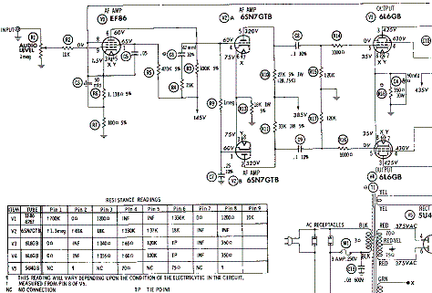
The wires to the vacuum tubes (the globes labelled V1 through V5) are labelled with voltages, and the table in the lower left corner that lists the correct resistances that will hold at each of the wires (``pins'') that connect to the tubes.
The voltage and resistance calculations are an analysis and a prediction of the circuit's behavior. The numbers were calculated with mathematics and algebra, and if the electronics parts are working correctly, then these voltage, amperage, and resistance levels must occur.
A computer program is a ``circuit'' that ``runs on'' knowledge, and when we design the parts (lines) of a computer program, we should include ``knowledge checks'' that assert the amount of knowledge computed by the program at various points.
This little program
selects the larger of two integers and prints it:
x = readInt()
y = readInt()
if x > y :
    max = x
else :
    max = y
print max
Pretend the program is a ``circuit'' where
information or knowledge ``flows'' from one line to the next.
Here is the program's ``schematic'' where the internal ``knowledge levels''
are written in symbolic logic and are inserted within the lines
of the program, enclosed by set braces, { ... }:
===================================================

x = readInt()
y = readInt()
if x > y :
    { 1. x > y     premise  }
    max = x
    { 1. x > y     premise
      2. max == x  premise
      3. max >= x  algebra 2
      4. max >= y  algebra 1 3
      5. max >= x  ∧  max >= y   ∧i 3 4
    }
else :
    { 1. ¬(x > y)       premise
      2. y >= x       algebra 1
    }
    max = y
    { 1. max == y    premise
      2. y >= x      premise
      3. max >= y    algebra 1
      4. max >= x    algebra 1 2
      5. max >= x  ∧  max >= y   ∧i 4 3
    }

{ 1. max >= x  ∧  max >= y   premise  }
print max

===================================================
The last annotation, { max >= x ∧ max >= y }, is the
symbolic-logic statement that max is guaranteed to be greater-or-equal
to both inputs. We now know, once the program is implemented,
it will behave with this logical property.
=================================================== AND:The input wires are labelled with the names P and Q. The output is emitted from the rightmost wire that exits the gate. The gates' physical behaviors are summarized by truth tables:OR:
NOT:
===================================================
AND: P Q |       OR: P Q |        NOT: P |
-------------    ------------     -----------
     t t | t         t t | t           t | f
     t f | f         t f | t           f | t
     f t | f         f t | t
     f f | f         f f | f
We use t (read ``true'')
for high voltage and f (read ``false'') for low voltage.
We write each gate in a linear notation,
that is, instead of drawing
,
we write P ∧ Q instead.
The notations are
AND  is  ∧
OR   is  ∨
NOT  is  ¬
We can compose the gates to define new operations.
For example, this circuit,
written ¬(P ∧ Q), defines this computation of outputs:
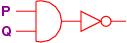
     P Q | ¬ (P ∧ Q)
    -------------------------
     t t | f     t
     t f | t     f
     f t | t     f
     f f | t     f
(Notice that the circuit's output is written in the column
underneath the NOT symbol, ¬, which is the outermost (last)
operator/gate in the circuit.
We said that voltage levels
travel along the wiring of a circuit. But we can also
argue that it is knowledge that travels the circuit.
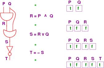
Here is a circuit:
and here is its coding in an equational, hardware description language:
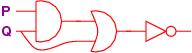
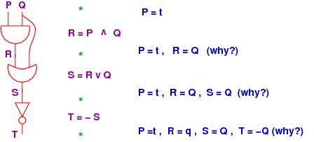
R = P ∧ Q
S = R ∨ Q
T = ¬ S
Let's redraw the circuit vertically and lay it side by side with
the assignment equations:
===================================================
Now, at each of the program points, marked by stars,
what information is kept in the wires?
 ===================================================
===================================================
The wiring diagram shows the values on the wires labelled
P, Q, R and S
as they travel through the circuit. But this is just tracking
the values of the variables in the assignment program we wrote!
 ===================================================
What if we don't know what Q will be? Say that P is t. What can we
calculate about the circuit anyway? It's this:
===================================================
In the diagram, we see that R = Q is stated after the
AND gate. How do we know this?
 ===================================================
First, we do know that R = P ∧ Q. But P = t. We substitute t for P and obtain R = t ∧ Q. Next, we do a cases analysis and consider the cases of Q's possible value: If Q is t, then t ∧ Q is t ∧ t, which simplifies to t, that is, to Q's value. Similarly, when Q is f, then t ∧ Q is f as well. Hence, in both cases, t ∧ Q equals Q.
The above reasoning is a deduction --- we deduced from the facts P = t and R = P ∧ Q that R = Q.
The example shows that we can reason about what the circuit will do in terms of the design we followed. This idea generalizes nicely to computer programs that are ``circuits'' on numbers (and not just on true and false)!
===================================================In the 1970's, this form of circuit, called a data-flow program, was used with computers with multiple processors for parallel computation. Such circuits are now again being investigated for use with multi-core processors. Here is the equational system for the above circuit:===================================================
a = x + y b = 2 * a c = y + 1 d = b - cThis equation set uses one operation in each equation. It is called three-address code and is produced by a compiler when the compiler translates complex arithmetic expressions into machine language.
Let's repeat the exercise at the end of the previous section for
this equational system.
Say that we know nothing
about the values of ``inputs'' x and y, and we want to know
about d's ``output'' value in terms of just x and y. This calculation
is just algebra,
and it looks like this:
===================================================
a = x + y
therefore, a = x + y
b = 2 * a
therefore, a = x + y, b = 2 * a
and b = 2 * (x + y) by substitution
c = y + 1
therefore, b = 2 * (x + y), c = y + 1
d = b - c
therefore, b = 2 * (x + y), c = y + 1, d = b - c
and d = (2 * (x + y)) - (y + 1) by substitution
and d = 2x + y - 1 by simplification
===================================================
Here, we deduced the ``output property'' of d in terms of the
``inputs'' x and y ---
d = 2x + y - 1 holds true when all the equations are ``computed.''
This reasoning is similar to what we use when we write assignment
commands in a programming language.
===================================================
hours = 4
{ 1. hours == 4 premise }
minutes = hours * 60
{ 1. hours == 4 premise
2. minutes == hours * 60 premise
3. minutes == 240 algebra 1 2
}
print hours, minutes
===================================================
We numbered each reasoning step;
premises are facts that are immediate from
the assignment command or facts that were previously established.
In Line 3, we used algebra, like
in the previous section,
to deduce the result.
This is a ``circuit'' through which ``knowledge'' flows!
In languages like C and Python, a programmer can insert assert
commands into the program to force
that a logical property holds true during the execution:
===================================================
hours = readInt("Type an int > 2: ")
assert hours > 2
# execution reaches here _only if_ the value assigned to hours is > 2
minutes = hours * 60
# here, we _know_ that minutes > 120
print hours, minutes
===================================================
When the computer executes the program, it checks that the number
read and assigned to hours is indeed greater than 2. If it is,
the computer proceeds; if it is not, the computer halts the program
with an assert exception. We use the assert commands in
our analysis:
===================================================
hours = readInt("Type an int > 2: ")
assert hours > 2
{ 1. hours > 2 premise (from the previous assert) }
minutes = hours * 60
{ 1. hours > 2 premise (previous fact, unaltered)
2. minutes == hours * 60 premise (from the assignment)
3. minutes > 120 algebra 1 2
}
print hours, minutes
===================================================
When we reassign to the same variable, our reasoning goes wrong. Consider:
===================================================
hours = 4
{ 1. hours == 4 premise }
minutes = hours * 60
{ 1. hours == 4 premise
2. minutes == hours * 60 premise
}
hours = 5
{ 1. hours == 5 premise
2. minutes == hours * 60 (WRONG!)
}
===================================================
Another, famous example is this:
===================================================
{ 1. x > 0 premise }
x = x + 1
{ 1. x == x + 1 ?!!! }
===================================================
Programming is not algebra!
We must distinguish the new value of x from the ``old'' value:
===================================================
assert x > 0
{ 1. x > 0 premise }
x = x + 1
{ 1. x == xold + 1 premise (from the assignment)
2. xold > 0 premise (from the assert)
3. xold + 1 > 1 algebra 2
4. x > 1 subst 1 3 (substitute Line 1 into Line 3)
# Finally, we delete all assertions that mention xold ---
# only Line 4 carries forwards.
}
===================================================
The assignment law we just used looks like this:
{ ...
m. P
}
x = e
{ 1. x == [xold/x]e premise
2. [xold/x]P premise
...
n. Q (where Q must _not_ mention xold)
}
The notation, [xold/x]E, means we substitute
all occurrences of x within expression E by xold.
Here is one more example, where we
maintain the relationship between a quantity of coins
(USA ten-cent pieces --- "dimes")
and their monetary value;
===================================================
# the _invariant property_ is that money == dimes * 10 :
assert money == dimes * 10
{ 1. money == dimes * 10 premise }
# Say that one more dime is inserted into the bank:
dimes = dimes + 1
{ 1. dimes == dimesold + 1 premise
2. money == dimesold * 10 premise
3. dimesold == dimes - 1 algebra 1
4. money == (dimes - 1) * 10 subst 3 2
}
# The amount of money is less that what it should be; we fix this:
money = money + 10
{ 1. moneyold == (dimes - 1) * 10 premise
2. money == moneyold + 10 premise
3. moneyold == money - 10 algebra 2
4. money - 10 == (dimes - 1) * 10 subst 3 1
5. money == dimes * 10 algebra 4
}
# The invariant property is restored: money == dimes * 10
print dimes, money
===================================================
The proof explains why we wrote
the assignments as we did --- we wanted to maintain the logical
property that money == dimes * 10.
This would be critical if the above software was embedded in
a chip within a child's bank: when the child inserts a coin, this
activates the above code, which resets dimes and money so that
the invariant property is always holding true.
Invariant properties are central to the development of real-time software, which iteratively monitors the values of input sensors and adjusts program variables so that invariants are maintained.
===================================================
if x > y :
max = x
else :
max = y
===================================================
What can we assert when the command finishes?
First, when we analyze the then-arm, we have
===================================================
max = x
{ max == x }
===================================================
and when we analyze the else-arm, we have
===================================================
max = y
{ max == y }
===================================================
These two deductions imply that, when the conditional finishes,
one or the other property holds true:
===================================================
if x > y :
max = x
else :
max = y
{ max == x ∨ max == y }
===================================================
The knowledge producted by the command is the disjunction
(or) of the knowledge produced by each arm.
The intent of the conditional was to set max so that it holds the larger of x and y. The assertion we proved so far does not imply the desired goal. This is because we ignored a critical feature of a conditional command: By asking a question --- the test --- the conditional command generates new knowledge from the answer.
For the then arm, we have the new knowledge that x > y;
for the else-arm, we have that ¬(x > y), that is, y >= x.
We embed these assertions into the analysi
and conclude that, in both cases,
max holds the maximum of x and y:
===================================================
if x > y :
{ 1. x > y premise }
max = x
{ 1. x > y premise
2. max == x premise
3. max >= x algebra 2
4. max >= y algebra 1 3
5. max >= x ∧ max >= y ∧i 3 4
}
else :
{ 1. ¬(x > y) premise
2. y >= x algebra 1
}
max = y
{ 1. max == y premise
2. y >= x premise
3. max >= y algebra 1
4. max >= x algebra 1 2
5. max >= x ∧ max >= y ∧i 4 3
}
{ 1. max >= x ∧ max >= y premise (from the if-command) }
===================================================
A classic logic law, ∧i (and-introduction), combines two facts
into a compound fact.
Here is the schematic of the forwards law for conditionals:
{ ... P }
if B :
{ 1. B premise
2. P premise
... }
C1
{ ... Q1 }
else :
{ 1. ¬B premise
2. P premise
... }
C2
{ ... Q2 }
{ 1. Q1 ∨ Q2 premise }
The law shows that the conditional command is a ``circuit''
that ``forks'' and ``joins.''
A function is a ``mini-program'': it has inputs, namely the arguments assigned to its parameters, and it has outputs, namely the information returned as the function's answer. It acts like a logic chip, with ``input wires'' and ``output wires.''
Here is the format for writing a function:
===================================================
def reciprocal(n) : # HEADER LINE : LISTS NAME AND PARAMETERS
"""recip computes the reciprocal for n"""
{ pre n != 0 # PRECONDITION : REQUIRED PROPERTIES OF ARGUMENTS
post answer == 1.0 / n # POSTCONDITION : THE GENERATED KNOWLEDGE
return answer # VARIABLE USED TO RETURN THE RESULT
}
answer = 1.0 / n # BODY (no assignment to n allowed)
return answer
===================================================
The precondition states the situation under
which the function operates correctly, and the postcondition
states what the function has accomplished when it terminates.
The person/program who calls the function is not supposed to read the function's code to know how to use the function.
To call the function, we supply an argument that binds
(is assigned to) its parameter that makes the precondition true:
===================================================
a = readInt()
if a != 0 :
{ 1. a != 0 premise } (from the law for conditionals)
b = reciprocal(a)
{ 1. b == 1.0 / a premise } (from the successful function call)
===================================================
As our reward for establishing the precondition, we receive in
return the postcondition, stated in terms of a and b:
b == 1.0 / a.
Here is the precise statement of the law for functions:
===================================================
def f(x):
{ pre Qx (assertion Q mentions x)
post Rans,x (assertion R mentions ans and x)
return ans (the answer variable)
}
{ 1. Qx premise }
BODY # does not assign to x
{ ...
m. Rans,x (prove this}
}
return ans
===================================================
Here is the schematic for a correct call of the function.
===================================================
{ ... [e/x]Qx }
y = f(e) # y does not appear in e
{ 1. [y/ans][e/x]Rans,x premise
2.[yold/y]P premise
...
}
===================================================
In the Python language, every global variable that is updated
by a function must be listed in the global line that
immediately follows the function's header line. This is a good
practice that we will follow.
Here is a simple example:
===================================================
pi = 3.14159
c = 0
def circumference(diameter) :
{ pre diameter >= 0 ∧ pi > 3
post c = pi * diameter
}
global c # will be updated by this procedure
c = pi * diameter
. . .
d = readFloat("Type diameter of a circle: ")
assert d >= 0
{ 1. d >= 0 premise
2. pi == 3.14159 premise
3. pi > 3 algebra 2
4. d >= 0 ∧ pi > 3 ∧i 1 3
# we proved the precondition for circumference
}
circumference(d)
{ 1. c == pi * d premise } # we get its postcondition
print c
===================================================
Here is an example of
a module/class that models a bank account;
the variable's value must be maintained at a nonnegative value:
===================================================
# BankAccount module/class:
balance = 100 # the global variable
{ 1. balance == 100 premise
2. balance >= 0 algebra 1
}
# the global invariant:
{ globalinv balance >= 0 } # must be maintained!
def deposit(howmuch) :
"""deposit adds howmuch to balance"""
{ pre howmuch >= 0
post True }
global balance
{ 1. balance >= 0 premise # the globalinv holds on entry
2. howmuch >= 0 premise # the function's precondition
}
balance = balance + howmuch
{ 1. balance = balanceold + howmuch premise
2. balanceold >= 0 ∧ howmuch >= 0 premise
3. balance >= 0 algebra 1 2
}
# The global invariant is preserved at the procedure's exit.
def withdraw(howmuch) :
"""withdraw removes howmuch from balance"""
{ pre howmuch >= 0
post True }
global balance
{ 1. balance >= 0 premise # the globalinv holds on entry
2. howmuch >= 0 premise
}
if howmuch <= balance :
{ 1. howmuch <= balance premise }
balance = balance - howmuch
{ 1. balance = balanceold - howmuch premise
2. howmuch <= balanceold premise
3. balance >= 0 algebra 1 2
}
else :
{ 1. ¬(howmuch <= balance) premise
2. balance >= 0 premise
}
pass
{ 1. balance >= 0 pass }
{ 1. (balance >= 0) ∨ (balance >= 0) premise
2. balance >= 0) ∨e 1
}
# The global invariant is preserved at the procedure's exit.
===================================================
The two functions, deposit and withdraw, pledge to keep
balance nonnegative. Assuming that no other program
commands update the account, the proofs of the two functions
suffice to ensure that account's global invariant holds
always.
There are many examples of modules/classes that use global invariants: spreadsheet programs, board games, animations, .... You must use global invariants when you build realistic object-oriented programs!
If a loop is a ``function that restarts itself,'' then we ask, ``What are its pre- and post-conditions?'' Since the loop iterations follow one another, it must be that the postcondition from the end of the previous iteration is the exactly the precondition for starting the next iteration --- the loop's ``pre'' and ``post'' conditions are one and the same! The loop's pre-post-condition is called the loop's invariant. We can understand this with an example.
Consider the computation of factorial, which is
a repeated product: for integer n > 0,
n! == 1 * 2 * 3 * ...up to... * n
and it is traditional to define 0! = 1.
Here is a loop that computes the repeated product:
===================================================
n = readInt("Type a nonnegative int: ")
assert n >= 0
i = 0
fac = 1
while i != n :
i = i + 1
fac = fac * i
print n, fac
===================================================
The loop makes multiplications,
*1, *2, *3, etc., to the running total, fac, until
the loop reaches i == n.
Consider some execution cases:
0 times: fac = 1 = 0!
1 time: fac = 1 * 1 = 1!
2 times: fac = (1 * 1) * 2 = 2!
3 times: fac = (1 * 1 * 2) * 3 = 3!
4 times: fac = (1 * 1 * 2 * 3) * 4 = 4!
. . .
the loop repeats k+1 times: it computes fac = (k!) * (k+1) = (k+1)!
We deduce this fact upon the loop body like this:
===================================================
{ fac == i! } (we have conducted i iterations so far)
i = i + 1
{ 1. i == iold + 1 premise
2. fac == (iold)! premise
3. fac == (i-1)! algebra 1 2
}
fac = fac * i
{ 1. fac == facold * i premise
2. facold == (i-1)! premise
3. fac == (i-1)! * i subst 2 1
4. fac == i! definition of i!
}
===================================================
That is, the assertion that results from one more iteration is the same
as the assertion we had when we started the iteration!
This property holds true --- it is invariant for no matter
how many times the loop repeats.
If we think of a program as a circuit, where
knowledge flows along the ``wires'', then
a loop program is a feedback circuit, where knowledge, I,
is forced backwards into the circuit's entry:
I|
v
+->while B :--+
| I| |
| v |
| C v
I| |
+----+
The voltage (knowledge) level, I, must be stable along the back arc
of the circuit, else the circuit will ``oscillate'' and misbehave.
A loop works the same way --- for the loop to reach
its goal, there must be a stable level of knowledge
along the back arc --- its invariant.
When the loop for factorial quits, what do we know?
===================================================
n = readInt("Type a nonnegative int: ")
assert n >= 0
i = 0
fac = 1
{ i == 0 ∧ fac == i! }
while i != n :
{ fac == i! }
i = i + 1
fac == fac * i
{ fac == i! }
{ 1. i == n premise (the loop's test is False)
2. fac == i! premise (the invariant still holds)
3. fac = n! subst 1 2 (the loop accomplished its goal)
}
print n, fac
===================================================
Since the loop terminated its iterations at the correct time,
fac holds the correct answer.
Here is the law we use for deducing the properties of a while-loop.
It uses an invariant assertion, I:
{ ... I } (we must prove this True before the loop is entered)
while B :
{ invariant I }
{ 1. B premise
2. I premise
...
}
C
{ ... I } (reprove I at the end)
{ 1. ¬B premise
2. I premise
...
}
===================================================
def reverse(word) :
"""reverse reverses the letters in w and returns the answer"""
{ pre w is a string
post ans == w[len(w)-1] w[len(w)-2] ...down to... w[1] w[0]
return ans
}
===================================================
How to do it? Count through the letters of w and copy each letter
to the front of variable string ans. Iteration number i would go
ans = w[i] + ans i = i + 1When we apply this repeatedly, we get the desired behavior:
=================================================== after 0 iterations: w = "abcd" i = 0 ans = "" after 1 iteration: w = "abcd" i = 1 ans = "a" after 2 iterations: w = "abcd" i = 2 ans = "ba" after 3 iterations: w = "abcd" i = 3 ans = "cba" after 4 iterations: w = "abcd" i = 4 ans = "dcba" ===================================================The invariant is that the first i letters of w are found in reverse order within ans:
ans = w[i-1] w[i-2] ...down to... w[0]You should check that this is indeed an invariant property of the proposed loop body above. This completes the function:
===================================================
def reverse(w) :
"""reverse reverses the letters in w and returns the answer"""
{ pre w is a string
post ans == w[len(w)-1] w[len(w)-2] ...down to... w[1] w[0]
return ans
}
ans = ""
i = 0
{ 1. ans == "" premise
2. ans == w[i-1] w[i-2] ...down to... w[0] algebra 1
# ``-1 down-to 0'' is an empty range of characters from w
}
while i != len(w) :
{ invariant ans == w[i-1] w[i-2] ...down to... w[0]
modifies ans, i
}
ans = w[i] + ans
{ 1. ans == w[i] + ansold premise
2. ansold == w[i-1] w[i-2] ...down to... w[0] premise
3. ans == w[i] + w[i-1] w[i-2] ...down to... w[0] algebra 1 2
}
i = i + 1
{ 1. i == iold + 1 premise
2. ans == w[iold] + w[iold-1] w[iold-2] ...down to... w[0] premise
3. iold == i - 1 algebra 1
4. ans == w[i-1] w[i-2] ...down to... w[0] subst 3 2
}
{ 1. i = len(w) premise
2. ans == w[i-1] w[i-2] ...down to... w[0] premise
3. ans == w[len(w)-1] w[len(w)-2] ...down to... w[0] subst 1 2
} # the function's postcondition is proved
return ans
===================================================
We can construct this proof a bit more precisely with the assistance
of these two recurrences:
rev(w, ans, 0) if ans == "" rev(w, ans, k+1) if rev(w, a', k) and ans == w[k] + a'That is, rev(w, a, n) says that the first n letters of string w are saved in reverse order in string a, that is,
rev(w, a, n) exactly when a == w[n-1] + w[n-2] + ...downton... + w[0]Now, we need not depend on the ellipsis (...) in our deduction steps --- we use the two recurrence definitions to prove that the loop's invariant is rev(w, ans, i):
===================================================
{ def rev(w, ans, 0) if ans == ""
def rev(w, ans, k+1) if rev(w, a', k) and ans == w[k] + a'
}
def reverse(w) :
"""reverse reverses the letters in w and returns the answer"""
{ pre w is a string
post rev(w, ans, len(w))
return ans
}
ans = ""
i = 0
{ 1. ans == "" premise
2. rev(w, ans, 0) if ans == "" def
3. rev(w, ans, 0) ife 2 1 # ``if elimination''
4. i == 0 premise
5. rev(w, ans, i) subst 4 3
}
while i != len(w) :
{ invariant rev(w, ans, i)
modifies ans, i
}
ans = w[i] + ans
{ 1. ans == w[i] + ansold premise
2. rev(w, ansold, i) premise
3. rev(w, ansold, i) and ans == w[i] + ansold andi 2 1
4. rev(w, ans, i+1) if rev(w, a', i) and ans == w[i] + a' def
5. rev(w, ans, i+1) ife 3 4
}
i = i + 1
{ 1. i == iold + 1 premise
2. rev(w, ans, iold+1) premise
3. rev(w, ans, i) subst 1 2
}
{ 1. not(i != len(w)) premise
2. rev(w, ans, i) premise
3. i == len(w) algebra 1
4. rev(w, ans, len(w)) subst 3 2
} # the function's postcondition is proved
return ans
===================================================


===================================================
a = [5, 10, 15, 20, ... ]
i = 0
while i != len(a) :
{ invariant: ??? }
a[i] = a[i] * a[i]
i = i + 1
print a
===================================================
In words, the loop's invariant is that
``while the loop is running,
all of a's elements, from 0 up to i, are squared.''
It is a little difficult to state this precisely with algebra
notation. Our first attempt might read like this:
Let  ain be the starting value of a.  The invariant is

a[0] = ain[0] * ain[0]  ∧
a[1] = ain[1] * ain[1]  ∧
 ... ∧
a[i-1] = ain[i-1] * ain[i-1]  ∧
a[i] = ain[i]             ∧
a[i+1] = ain[i+1]         ∧
 ... ∧
a[len(a)-1] = ain[len(a)-1]
This is overly wordy.
There is a better way to represent the assertion, using the
logical operator, ``forall''. (We will see that the for-all
operator is written ∀, but for now we use the words, ``for all''.)
The invariant is
forall 0 <= j < i, a[j] = ain[j] * ain[j]
∧
forall i <= j < len(a), a[j] = ain[j]
That is, for all j in the range from
0 to i-1, a[j] = ain[j] * ain[j], and
for all j in the range, i to len(a)-1, a[j] = ain[j].
This indicates clearly that array a is split into the segment
from a[0] up to a[i-1], whose elements are squared, and the segment,
a[i] to the end, whose elements are not yet altered.
Notice that when the loop quits, it is because i == len(a).
In this situation, the range from i to len(a)-1 is empty, and the
segment of unaltered elements is also empty.
Many labs and shops use automated tools that do some or most of the analysis that is shown here, in the color green, in these notes. Examples of such tools are Spec#, Boogie, and ESC-Java, all used by Microsoft.
I have written a prototype tool you can use with the examples in these notes. You can download the tool and more material at my website, http://www.cis.ksu.edu/~schmidt/301f09.
The notes you have just read are found at http://www.cis.ksu.edu/~schmidt/papers/hometalks.