Chapter 8:
The logical paradigm: From a boolean core to Prolog

8.1 A logical core language: logical variables and backtracking
8.2 Predicate abstracts are Horn clauses
    8.2.1 Parameter patterns
    8.2.2 Functions and relations
8.3 Data structures: functors
    8.3.1 Data bases
    8.3.2 Lists
    8.3.3 Trees
    8.3.4 Matching versus unification
8.4 Control structures: findall
    8.4.1 Cut
8.5 No control structures: specifications are programs
8.6 Parser and interpreter construction with Prolog
8.7 A few additional useful Prolog predicates
8.8 An implementation you can use
8.9 Addendum: Adding storable values

When you solve a crossword puzzle or a Sudoku puzzle, you are confronted with a gameboard of empty squares and a set of clues. (In Sudoku, the clues are values already inserted in some of the squares.) You solve the puzzle by placing values in the empty squares so that they fit the clues. Maybe you make some guesses for some of the squares, and you guess incorrectly, so you must ``backtrack'' and erase the values you placed in the squares and try again. Ultimately, there is a ``correct'' value for each square, and once you find the value, it stays in the square permanently. The puzzle is solved when all the squares are filled correctly to match the clues.

There is a style of programming that matches puzzle solving --- it is called constraint programming or logical programming. In the logical-programming paradigm, a program (more precisely, a specification of a program) is a set of constraints, written as logical assertions, and a goal formula with "empty squares" (variables to be assigned to). A computation finds values for the variables in the goal formula so that all the assertions are made true.

The variables are called logical variables, and they are like the empty squares of a puzzle. The logical assertions are like the clues/constraints to the puzzle. The computation uses deductive techniques to discover combinations of values to bind to the logical variables, trying to make/prove the goal true. If a combination of values fails, the computation backtracks (erases some of the values from the logical variables) and tries other combinations.

For example, here is a goal: 2 + 1 = X. The X is a logical variable, a ``square'' to be filled to make the goal assertion true. If we bind 3 to X, we ``solve'' the ``puzzle.'' A puzzle can have more that one solution, for example, the goal assertion, Y > 3, can be solved by binding Y to 4 or to 5, etc.

In algebra class, you get puzzles like this:

X = 2 * Y
Y = Z
Z = 5        "Now, solve for X."

You guess values for X, Y, and Z, and you discover that 10 is the solution for X.

Here is an example of how logical assertions can help solve a goal. We have these two laws for integers:

(A > 0) -> ((2 * A) > A)    // "for any int A, if A is > 0, then so is 2*A"
3 > 0                       // " 3 is > 0"

Say the goal is again Y > 3. The second law above says that 3 > 0, and when combined with the first law, we deduce (2 * 3) > 3, meaning that Y == 6 is a solution to the goal.

The logical-programming paradigm is useful for solving problems in data bases, knowledge discovery, and learning: a data- or knowledge-base is coded as a set of logical assertions, and a query to the database is a logical assertion with variables that must receive values to answer the query. The paradigm is also useful to a non-programmer who can write down the laws of their problem domain as logical assertions and then ask questions in logical-formula-form.

In this chapter, we study the structure of Prolog, the most popular language in the logical-programming paradigm.

8.1 A logical core language: logical variables and backtracking

A core language for a logical language should define how to write logical assertions. Here is the syntax we use; it is a variant of propositional logic:

===================================================

A: Atom (a single-quoted string)
X: LogicalVariable (a string that begins with an upper-case letter)
E: Element  (expressions)
P: Proposition (logical assertions)
Q: Query

Q ::=  ?- P .
E ::=  A  |  X
P ::=  E1 = E2  |  P1 , P2  |  P1 or P2  |  true  |  false
A ::=  a single-quoted string

===================================================

The ``expressions'' of this language are elements, which, for the moment, are primitive atoms (strings) or variables. Logical assertions are expressed as predicates which are either equality assertions, conjunctions (P1, P2 stands for ``P1 ∧ P2''), disjunctions, or just the primitives, true and false. (IMPORTANT: in the Prolog language, or is coded by ;.)

A program is a query, that is, a proposition that must be made true by binding values to the logical variables (that is, by "solving for the variables"). The ``answer'' to the query (program) is the set of bindings that make the query true.

For this core language, the expressible values are strings; the denotable values are the expressibles; and there are no storables, because there is no storage structure and no assignments.

Think of a query in this language as a puzzle that must be solved; it is a goal to be achieved. For example, the query,

?-  X = 'abc'.

asks us to solve for X, and the solution is binding 'abc' to X. The answer to the query, the result of the computation, is the binding set (environment), {X == 'abc'}

Here are more examples:

?- X = 'kim' or X = 'icecream' .
This goal can be achieved in two ways. The first solution sets X to 'kim', that is, the answer is the environment, {X == 'kim'}. A second solution sets X to 'icecream', that is, {X == 'icecream'}.
?- X = 'kim', X = 'john'.
This goal cannot be achieved, because variable X must be simultaneously bound to both kim as well as john, and this is impossible. The result is false.
The query
?- Y = Y
returns true, because no binding was needed to make the query true; the answer environment is { }.
?- (X = 'john', (Y = 'icecream' or Y = 'mary')) or (X = 'mary') .
This query can be solved in three ways. Let's say that the interpreter reads the query from left to right:
1. Since the goal has the form, P or Q, one approach makes the P-part true:
  X = 'john', (Y = 'icecream' or Y = 'mary')
  This subgoal has form ``R and S'', so an environment (solution) must be found that makes both R and S true. The X = 'john'-part builds the environment, {X == 'john'}, which is carried forward to solve the second goal. We will write it like this:
  {X == 'john'} ?- Y = 'icecream' or Y = 'mary'
  This subgoal can be solved by solving its first disjunct:
  {X == 'john'} ?- Y = 'icecream'
  Here is the first solution: {X == 'john', Y == 'icecream'}.
2. The second solution is found by ``pretending'' that the first solution failed. That is, we erase Y == 'icecream' and revert (backtrack) to the environment, {X == 'john'} and solve the second disjunct:
  {X == 'john'} ?- Y = 'mary'
  This gives the second solution: {X == 'john', Y == 'mary'}.
3. To discover the third solution, we pretend that neither the first nor second solutions worked and proceed from there. This means we backtrack all the way back to the original disjunction, (X = 'john', (Y = 'icecream' or Y = 'mary')) or (X = 'mary') and try to prove its second disjunct:
  {} ?- X = 'mary'
  This gives the third solution: {X == 'mary'}
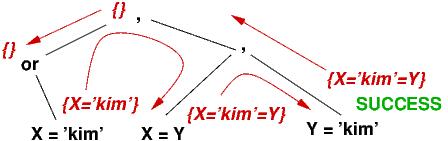
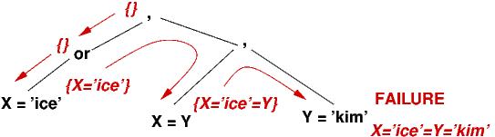
The example shows that the interpreter solves a query from left to right. To find more solutions, if any exist, the interpreter pretends that the solution failed, and it backtracks --- each occurrence of or offers another possibility for solving the query.
This example shows why the environment is critical to solving a query:
?- (X = 'icecream' or X = 'kim'), X = Y, Y = 'kim' .
The interpreter must solve three subgoals: X = 'icecream' or X = 'kim' and then X = Y and then Y = 'kim'. Here are the steps:
1. {} ?- X = 'icecream' or X = 'kim'
  This computes {X == 'icecream'}.
2. Next,
  {X == 'icecream'} ?- X = Y
  This computes {X == 'icecream' == Y}.
3. Now there is trouble:
  {X == 'icecream' == Y} ?- Y = 'kim'
  It is impossible to augment the environment so that 'icecream' == Y == 'kim' --- the search has failed.
4. The interpreter backtracks to the most recent disjunction, X = 'icecream' or X = 'kim'. This time, the second disjunct is solved:
  {} ?- X = 'kim'
  This generates {X == 'kim'}.
5. The following subgoals, X = Y and Y == 'kim', can be solved with the environment, {X == 'kim'}, generating the solution, {X == 'kim' == Y}.

For all these examples, we can draw search trees that show how the environments are built while searching for a solution. In the last example, Steps 1-3 generate this search tree:
after the backtracking, the search Steps 4 and 5 look like this:

8.2 Predicate abstracts are Horn clauses

If the same proposition is needed over and over, we might want to name it. Here is the syntax of predicate abstracts, equipped with element (expression) parameters:

===================================================

S: Session
D: Definition

S ::=  D  ?- P .
D ::=  D1 D2  |  I1(I2*) :- P .
P ::=  ...  |  I(E*)

===================================================

As usual, I* means zero or more identifiers, separated by commas, and E* means zero or more expressions, separated by commas. Abstracts are listed in a sequence, terminated by periods. The meaning of a call, I(E*), is the binding of the arguments to I's parameters, augmenting the environment with the bindings.

Here is a simple example that defines two abstracts followed by a query:

===================================================

expensive(X) :- (X = 'house') or (X = 'car').
likes(Y, Z) :- Y = 'john',  expensive(Z).
?- likes('john', B).

===================================================

The first abstract states that when X is bound to 'house' or 'car', then the result is true (``a house is expensive; a car is expensive''). The second abstract returns true if its first argument is 'john' and its second argument makes expensive compute to true (``john likes Z if Z is expensive'').

Here's how the interpreter searches for a solution to likes('john', B) ("What does john like?"):

===================================================

  {} ?- likes('john', B) : Ans0     (Ans0 will be the answer environment.)

Execute the call to  likes  and bind arguments to parameters:
  {Y == 'john', B == Z} ?-  Y = 'john', expensive(Z) : Ans0

The prover must solve the left conjunct and pass the solution
to the right conjunct:

  {Y == 'john', B == Z} ?-  Y = 'john' : Ans1

  Ans1 ?-  expensive(Z) : Ans0

The first conjunct is already solved:   Ans1 ==  {A == Y == 'john', B == Z}    

To complete the call to  likes,  we solve the other subgoal:

  {Y == 'john', B == Z} ?- expensive(Z) : Ans0

Execute the call to  expensive and bind the argument to the parameter:

  {Y == 'john', B == Z == X} ?-  (X = 'house') or (X = 'car') : Ans0

Try to solve left disjunct:
  { Y == 'john', B == Z == X}  ?-  X = 'house' : Ans0

Succeeds:  Ans0 == {Y == 'john', B == Z == X == 'house'}

===================================================

The solution is displayed as B == 'house'
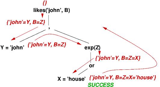
(The internal variables are not displayed.) Here is the search tree for the above deduction steps:

===================================================

exp(X) :- (X = 'house') or (X = 'car').
likes(Y, Z) :- Y = 'john',  expensive(Z).
?- likes('john', B).


===================================================

There is a second solution, which is found by pretending the last-chosen disjunct was a failure. This backtracks to the most recent or in the execution sequence:

===================================================

Backtrack to
  {Y == 'john', B == Z == X} ?-  (X = 'house') or (X = 'car') : Ans0

and try to solve the right disjunct:
  {Y == 'john', B == Z == X}  ?-  (X = 'car') : Ans0

Succeeds:  Ans0 == {Y == 'john', B == Z == X == 'car'}

===================================================

There are no more disjuncts to try, so the search is exhausted.

In the example, the parameter variables are just logical variables. We were lucky that all the parameter variables were distinct. This isn't always true, so each time an abstract is called, the interpreter creates new variable names for the formal-parameter variables. This avoids confusion. For example:

expensive(X) :- (X = 'house') or (X = 'car').
likes(X, Z) :- X = 'john',  expensive(Z).

Here is how it's done: prove ?- likes(A, B) ("Who likes what?")

===================================================

  {}  ?- likes(A, B) : Ans0

  {X0 == A,  Z0 == B}  ?-  X0 = 'john',  expensive(Z0)  : Ans0

Equate  X0  with  'john':

  {X0 == A == 'john', Z0 == B}  ?- expensive(Z0) : Ans0

Note the distinct parameter name generated for the call to  expensive:

  {X0 == A == 'john', Z0 == B ==  X1} ?-  (X1 = 'house') or (X1 = 'car') : Ans0

This succeeds with  {X0 == A == 'john', Z0 == B == X1 == 'house'}
and also with       {X0 == A == 'john', Z0 == B == X1 == 'car'}

===================================================

As you have probably guessed, the two functions we have been using are both strategies and also logical formulas:

expensive(X) :- (X = 'house') or (X = 'car').
To prove something is expensive, prove it is a house or car:
∀X((X = 'house' ∨ X = 'car') —> expensive(X))
likes(Y, Z) :- Y = 'john', expensive(Z).
To prove that someone likes something, prove that the someone is john and the something is expensive:
∀X∀Z((X = 'john' ∧ expensive(Z)) —> likes(X, Z))

The functions are called Horn clauses. The query, ?- likes(A, B), is written in logic like this: ∃A∃B(likes(A,B))
To prove the query true, the interpreter searches for values (witnesses, as they are called in logic) that show there do indeed exist values, A and B, such that likes(A,B).

Here is a second example. The one abstract that follows codes all these facts:

--- john likes icecream and mary

--- everyone likes kim

--- ed likes everything

These facts are summarized in a relationship named, likes. Read the the following as, ``X likes Y if....''

===================================================

likes(X, Y) :- (X = 'john', (Y == 'icecream' or  Y == 'mary'))
               or (Y = 'kim')
               or (X = 'ed').

===================================================

We might make this query: ``who likes icecream?'' as ?- likes(Z, 'icecream').
The two solutions are Z == 'john' and Z == 'ed'. Here, icecream is the ``input'' argument to ``function'' likes and Z is the ``output'' variable.

Another query is, ``what does john like?'' --- likes('john', X). Here, john is the input and X gets the output. (The three outputs for X are icecream, mary, and kim.)

The query, likes('john', 'mary') returns true (no assignments to the empty environment are necessary). Both arguments are inputs. The query, likes('john', 'john') returns false. Finally, likes(A,B) returns all the combinations embedded within the rule for likes; both variables are output variables.

Here is another example, which lists which individuals (atoms) are female, which individuals have which parents, and what it means for one individual to have a second as a sister:

===================================================

female(X) :- X = 'marge' or X = 'lisa' or X = 'maggie' .

parents(A, B, C) :- B = 'homer', C = 'marge',
                    (A = 'bart' or A = 'maggie' or A = 'lisa') .

sisterOf(X,Y) :- female(Y), parents(Y,M,W), parents(X,M,W).

===================================================

(Read the second abstract as defining when A has B and C as parents; read the third as saying that X has Y as a sister.) The abstracts define a database that can be queried: ?- sisterOf('bart', B).
Let's follow the steps the computation takes to discover the first solution, B == 'lisa':

===================================================

{} ?-  sisterOf('bart', B) : Ans0

{X0 == 'bart', B == Y0} ?-  female(Y0), parents(Y0,M0,W0), parents(X0,M0,W0) : Ans0

{X0 == 'bart', B == Y0} ?- female(Y0) : Ans1

{X0 == 'bart', B == Y0 == X1} ?-  X1 = 'marge' or X1 = 'lisa' or X1 = 'maggie' : Ans1

Set  Ans1 == { X0 == 'bart', B == Y0 == X1 == 'marge'}

Ans1 ?- parents(Y0,M0,W0) : Ans2

Set Ans2 == {X0 == 'bart', B ==  Y0 == X1 == 'marge',
             A2 = 'marge', B2 == M0, C2 == W0}

Ans2 ?-  B2 = 'homer', C2 = 'marge',
         (A2 = 'bart' or A2 = 'maggie' or A2 = 'lisa') : Ans0

This fails, because there is no consistent assignment to  A2 ---
there is no proof of  'marge's parents.


Backtrack to the disjunction and try the next option:

{X0 == 'bart', B == Y0 == X1}  ?- X1 == 'lisa' : Ans1

Set Ans1 == {X0 == 'bart', B == Y0 == X1 == 'lisa'}

These two subgoals will now be proved:

Ans1 ?- parents(Y0,M0,W0) : Ans2
Ans2 ?- parents(X0,M0,W0) : Ans0

Ans0 ==  {X0 == 'bart', B ==  Y0 == X1 == 'lisa' == A2,
          B2 == M0 = 'homer', C2 == W0 == 'marge'}
This succeeds.

===================================================

The interpreter first tried to prove that female marge is bart's sister, but it could not prove that marge has parents, so the attempt failed. A backtrack discovers that female lisa has parents and these parents match bart's.

The previous definition of sisterOf is a bit imprecise, because it allows the Prolog interpreter to prove that every female with parents is a sister of herself. To remove this faulty conclusion, we can add a not-equals requirement, \=, like this:

sisterOf(X,Y) :- female(Y), parents(Y,M,W), parents(X,M,W), X \= Y.

The subgoal, X \= Y, is proved true if X and Y have distinct, nonequal values. You can also use = to check for equality.

Strategies for proving

Here are the strategies that were used in the previous examples:

===================================================


env ?- p(e1, e2, ...) : Ans
----------------------------------------------- where  p(X1, X2, ...) :- body
env U {X1 == e1, X2 == e2, ...} ?- body : Ans


env ?- g1 or g2 : Ans                env ?- g1 or g2 : Ans 
-------------------------            -------------------------
env ?- g1 : Ans                      env ?- g2 : Ans


env ?- g1 , g2 : Ans
----------------------------------------
env ?- g1 : Ans1     Ans1 ?- g2 : Ans


env ?- X == v : Ans
------------------------------------------ if (X == v') not in env,  
SUCCEEDS, where  Ans == env U {X == v}        for Atoms  v != v'

===================================================

These form the control algorithm of a Prolog interpreter.

8.2.1 Parameter patterns

In the previous chapters, we saw that abstracts become more readable if patterns can be used in place of simple formal-parameter names. Patterns are useful here, too. For example, these abstracts,

===================================================

likes(X, Y) :-  (X = 'john', sweet(Y))
                or (X = 'ed')
                or (Y = 'kim').
sweet(Z) :-  Z == 'icecream' or  Z == 'mary'

===================================================

can be split into clauses definition, where the parameter names are replaced by atomic patterns:

===================================================

likes('john', Y) :-  sweet(Y).
likes('ed', Y) :- true.
likes(X, 'kim') :- true.
sweet('icecream') :- true.
sweet('mary') :- true.

===================================================

This is more readable than the original definitions. We can also employ a Prolog abbreviation that drops true and the quotes around the atoms. This gives us Prolog's syntax for abstracts:

===================================================

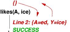
likes(john, Y) :-  sweet(Y).
likes(ed, Y).
likes(X, kim).
sweet(icecream).
sweet(mary).

===================================================

The clauses list all the disjuncts in the original definitions, one disjunct per line, which is easier to read. It is also easier to deduce answers to queries, e.g., ``who likes icecream?'':

===================================================

{} ?- likes(A, icecream) : Ans0

      (try the first clause:)

{} ?- likes(john, Y) : Ans0   

      (this expands to:)

{A == john, icecream == Y} ?- sweet(Y) : Ans0

This subgoal succeeds with Clause 4, provided that  Y == icecream, which it does.
So,  Ans0 == {A == john, icecream == Y}

===================================================

Note that the subgoal, {A == john, icecream == Y} ?- sweet(Y) : Ans0, fails with Clause 5, which requires that Y == mary.

Another answer to {} ?- likes(A, icecream) is of course {A == ed, Y == icecream}.

The search trees for the above solutions are remarkably small:

===================================================

(1) likes(john, Y) :- sweet(Y).             (4) sweet(ice).
(2) likes(ed, Y).                           (5) sweet(mary).
(3) likes(X, kim).
       

===================================================

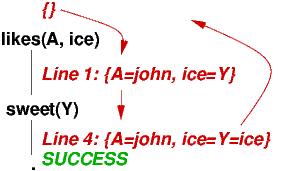
The example of females, parents, and sisters is also simplified by coding it in Prolog style:

===================================================

female(marge).
female(lisa).
female(maggie).

parents(bart, homer, marge).
parents(lisa, homer, marge).
parents(maggie, homer, marge).

sisterOf(X,Y) :- female(Y), parents(Y,M,W), parents(X,M,W), X \= Y.

===================================================

8.2.2 Functions and relations

You have likely noticed that a query like ?- likes('john', B) is a kind of ``function call'' that ``computes'' an answer for the ``output parameter variable'' B. This is indeed how one imitates conventional C-style functions in Prolog --- as predicates that have ``input arguments'' and ``output variables''. For example, these clauses likes(john, Y) :- sweet(Y). sweet(icecream).
might be read as two functions: # returns something that who likes: def likes(who) : if who == 'john' : return sweet() def sweet() : return 'icecream'
so that a call to likes('john') returns 'icecream' as an answer.

But Prolog clauses act like a function that can return ``more than one answer'', e.g.,

likes(john, Y) :-  sweet(Y).
likes(X, kim).
sweet(icecream).
sweet(mary).

Now it is possible for some individuals (here, john) to like more than one atom. This might be faked with functions and lists: # returns a list of what who likes: def likes(who) : if who == 'john' : return sweet() + ['kim'] else : return ['kim'] def sweet() : return ['icecream', mary']
But this function mimickry breaks down when we encounter clauses like these: likes(john, Y) :- sweet(Y). likes(X, kim). likes(ed, Y). sweet(icecream). sweet(mary).
Since ``ed likes everything,'' there is no corresponding function coding.

Further, there is no easy way to ``run a function backwards'' to match a query like this,

?- likes(A, icecream)

which asks which arguments lead to an output of icecream. And this query, ?- likes(A, B).
generates all possible argument, output pairs for liking.

So, the clauses in Prolog go beyond function parameters --- they establish relationships between arguments ("john likes icecream"; "ed likes kim"; "icecream likes kim"), where there are no inherent "input" or "output" values.

When we write computations based on relationships, we are doing relational programming.

But if you are reluctant to leave the land of functions that have inputs and outputs, you can think of a Prolog clause as a "flexible function" where you choose which argument positions are inputs and which positions are outputs. For example, ?- likes(A, icecream), lets the first position be the output and the second be the input.

We will use these techniques in the following sections when we model and compute upon data structures.

8.3 Data structures: functors

In object languages, we use structs (dictionaries) as containers for data; in functional languages, we use layered/level data structures like lists and trees. In Prolog-like, relational languages, a data structure is a kind of labelled tuple-object. For example, given the atoms, 'Tale of Two Cities' and 'Charles Dickens', we build the new individual, book('Tale of Two Cities', 'Charles Dickens'). The data structure is a kind of struct that holds two fields, but it is also a kind of ML-like data structure. The constructor name, book, is called a functor in Prolog. (It is part function name, part constructor name.)

Since our language does not have data type names in its syntax, we can add the data-structure syntax directly to the syntax for Element:

===================================================

P: Predicate
E: Element (expressions)
f: Functor (data-structure constructors)
N: Numeral          A : Atom (string)

E ::=  A  |  X  |  f(E,+)  |  N  |  E1 + E2
P ::=  ...  |  E1 < E2  |  E1 =< E2

===================================================

f(E,+) is the syntax for a data structure, where E,+ stands for one or more elements separated by commas. We have also added numerals, N, and arithmetic addition, E1 + E2 as elements. We will compare numeric values with predicates like E1 < E2 and E1 =< E2.

We will go straight to examples.

8.3.1 Data bases

Functors are useful for defining records (structs) in databases. Perhaps a library will stock books and DVDs. In the library's database, these are represented by book(Title, Author) and dvd(Title), respectively. Here are two sample items:

book('David Copperfield', 'Charles Dickens')

dvd('Tale of Two Cities')

If the library owns an item, it is asserted with the predicate, owns(IdKey, Item), where Ikdey is the identification key for the Item. Here is a sample data base:

===================================================

owns('id90', book('David Copperfield', 'Charles Dickens')).
owns('id91', book('Tale of Two Cities', 'Charles Dickens')).
owns('id92', book('Tale of Two Cities', 'Charles Dickens')).
owns('id93', dvd('Tale of Two Cities')).
owns('id94', book('Moby Dick', 'Herman Melville')).

===================================================

When a patron borrows an item, an assertion of the form, borrows(IdKey, PatronName, TodaysDate), is added to the data base:

===================================================

borrowed('id92', 'Homer', 44).
borrowed('id93', 'Homer', 46).
borrowed('id91', 'Lisa', 92).
borrowed('id90', 'Lisa', 92).

===================================================

(The date could itself be a data structure of form, date(Day, Month, Year), but we use single ints for simplicity here.)

Here are some sample queries of the data base:

What items have Homer borrowed? (Don't display the date borrowed.) ?- borrowed(K, 'Homer', _). K = 'id92' K = 'id93'
In Prolog, _ stands for a ``logical variable'' whose value is not displayed when the answer environment is printed:

===================================================

GOAL                                ENVIRONMENT
---------------------------------------------------------
                                    { }

borrowed(K, 'Homer', _A)   # _A is an internal logical variable

# matches  borrowed('id92', 'Homer', 44):
                                    {K == 'id92', _A == 44} 

===================================================

What are the titles of books (not DVDs) that Homer borrowed? ?- borrowed(K, 'Homer', _), owns(K, book(T, _)) K = 'id92', T = 'Tale of Two Cities'
Here is how the solution is found:

===================================================

GOAL                                ENVIRONMENT
---------------------------------------------------------
                                    { }

borrowed(K, 'Homer', _A), owns(K, book(T, _B))

# solve the first subgoal:
borrowed(K, 'Homer', _A)
# matches borrowed('id92', 'Homer', 44):
                                   {K == 'id92', _A == 44}
# solve the second subgoal:
owns(K, book(T, _B))
# unifies with  owns('id92', book('Tale of Two Cities', 'Charles Dickens')) :

                                   {K == 'id92', _A == 44,
                                    T == 'Tale of Two Cities',
                                    _B == 'Charles Dickens'}

===================================================

When the second subgoal is solved, there is a ``two-way matching'' (unification) of the logical variables in the goal with the logical variables in predicate abstract. Note also that the _ symbol is a ``dummy variable'' that we do not care about --- its value is not printed. (Here we do not care about the book's due date nor the title and authors, so two dummy variables are used in the query.)

A unification can cause a logical variable to be bound to a data structure, e.g., the query, ``what items did Homer borrow?''
?- borrowed(K, 'Homer', _), owns(K, I).
is solved by these two environments:
K = 'id92', I = book('Tale of Two Cities', 'Charles Dickens') K = 'id94', I = dvd('Tale of Two Cities')

Librarians want to track overdue items. Here is a law for proving when a borrowed item is overdue. (Assume an item can be borrowed for two weeks.) /* isOverdue(Key, Today) holds true if Key is borrowed and its borrowed date is more than 14 days ago. */ isOverdue(Key, Today) :- borrowed(Key, Person, BDate), Today > BDate + 14. ?- isOverdue(K, 58). K = 'id92'

8.3.2 Lists

The list data structure is built into Prolog. A list is either empty, nil, or consists of an element, h, appended to the front of t, an existing list, h::t. In Prolog, nil is written [] and h::t is written [h|t].

Prolog's lists are like Python's lists: they can mix values, and lists can be placed within lists:

[a, b, c]

[2,4,6,eight]

['Homer', book('Tale of Two Cities', 'Charles Dickens')), book('Moby Dick', 'Herman Melville')) ] 

['Homer', [ book('Tale of Two Cities', 'Charles Dickens')),
            book('Moby Dick', 'Herman Melville')) ] ]

[]

The list builder, [_,_, ..., _], is a functor, just like book(_,_) and dvd(_), seen in the previous section.

Prolog uses the [H|T] pattern to compute on lists. Here is a trivial example: defining the front element of a list:

/* isFirst(D, L)  holds true if  D  is the front element of list L.  */
isFirst(D, [D|Rest]).

We use the ``function'' like this: ?- isFirst(X, [a,b,c]). X = a. ?- isFirst(X, []). false.
We can use recursion to define a property of all the elements in a list. Here is a simple, famous example:

===================================================

/* member(V, L)  holds true if  V  is an element of list  L.  */
member(V, [V|_]).
member(V, [_|T]) :- member(V, T).
member(V, []) :- fail.    # or omit it

===================================================

We can test the clauses with this example: ?- member(c, [a,b,c]).
Here's what happens:

To prove {} ?- member(c, [a,b,c]), the interpreter tries to match the first clause. This fails, because atom c is not the same as atom a within list [a,b,c]. (More precisely, the match, {V0 == c == a}, is impossible.)
The next clause is tried, matching against member(V, [_|T]). This match succeeds, and the interpreter tries to solve the subgoal, {V0 == c, T0 == [b,c]} ?- member(V0, T0).
To prove goal member(V0,T0) (that is, member(c,[b,c])), a match is attempted against member(V, [V|_]). This fails.
But the second clause matches a second time, and the new subgoal is
```
{V0 == c == V1, T0 == [b,c], T1 == [c]} ?- member(V1, T1)
```
(Notice how new parameter variables are generated for each new "call" to member so there is no confusion between the multiple calls.)
Finally, the goal, member(V1, T1) (that is, member(c,[c])), matches against the first clause, where
```
{V0 == c == V1 == V2, T0 == [b,c],
                      T1 == [c],
                      T2 == []}
```
There are no more subgoals to prove --- success! So
?- member(c, [a,b,c]). true

For fun, try these queries with Prolog: ?- member(X, [a,b,c]). ?- member(a, L). ?- member(X, L).
By the way, member is built into all Prolog implementations. Another built-in predicate is list append, which defines how two lists are appended together: /* append(L1, L2, M) holds true if list M is exactly list L1 appended to list L2 */ append([], L2, L2). append([H|T], L2, [H|A]) :- append(T, L2, A). ?- append([1,2], [a,b,c], A). A = [1,2,a,b,c].
Try these tests of append --- you might be surprised at the results!

?- append(A, [b,c], [1,2,b,c]). Which argument, when paired with [b,c], yields an ``answer'' of [1,2,b,c]?
?- append(A, B, [1,2,b,c]). Which argument combinations yield an ``answer'' of [1,2,b,c]?
?- append([1,2], B, C). What is the form of ``answer'' that arises when [1,2] is used as the first argument?
?- append([1|Rest], B, [1,2,3|More]). What combinations satisfy these restrictions on ``inputs'' and ``outputs''?

The examples show that any of append's three arguments might be used as ``inputs'' or as ``outputs.'' You can use Prolog clauses in this way to ``run programs backwards,'' calculate ``restrictions'' on inputs-outputs, etc.

Next, here are examples that work as ``functions'' on lists on numbers. The first sums a list of ints:

===================================================

/* totals(L, N)  holds if  L  is a list of ints and  N  is a sum of  L's ints */
totals([], 0).
totals([N|Rest], Answer) :- totals(Rest, Subanswer),
                            Answer is N + Subanswer.

?- total([1,2,3,4], A).
A = 10.

===================================================

Here, the pattern, [N|Rest], and the recursion, totals(Rest, Subanswer), systematically sum the shorter list and use the Subanswer to compute the entire sum.

Here is another example:

===================================================

/* double(L, M)  holds true if  L  is a list of ints and  M  is a list of
    ints whose values are exactly those of  L  multiplied by 2.  */
double([], []).
double([H|T], [HH|TT]) :-  HH is 2 * H,  double(T, TT).

?- double([1,2,3], A).
A = [2,4,6].

===================================================

If we pretend that double is a ``function'', then its first argument is its ``input'' and its second is its ``output.'' Notice how list patterns define the values of both the first (input) and second (output!) arguments. The use of patterns to construct ``outputs'' is unique to Prolog.

Finally, here is a "function" that inserts an int into its proper position of a list of ordered ints, e.g., insert(4, [1,3,5], Ans) will bind Ans = [1,3,4,5]:

===================================================

/* insert(N, L, NewL)  holds true if  L  is an ordered list of ints
     and list  NewL  is an ordered list of ints that has all of  L
     along with int  N   inserted in the proper position.  */
insert(N, [], [N]).
insert(N, [H|T], [N|[H|T]]) :-  N =< H.
insert(N, [H|T], [H|Subans]) :-  N > H, insert(N,T,Subans).

?- insert(4, [1,3,5], Ans)
Ans = [1,3,4,5].

===================================================

The example shows that list patterns can be nested ([N|[H|T]]). Notice also that the comparisons, N =< H and N > H, act as ``if-tests'' so there is no need for an if-else construction in Prolog.

8.3.3 Trees

In an ML-like functional language, a data structure is defined by a grammar rule called a datatype. Recall from the previous chapter that the data type of trees is defined with a leaf data structure and a node data structure. A tree data structure is either

a leaf, of

a node, node(E, T1, T2), where E is an element and T1 and T2 are other tree data structures.

In ML, we declare the tree data type like this: datatype Tree = Leaf | Node of Atom * Tree * Tree
In Prolog, there is no need for the datatype equation --- we just build the phrases, leaf and node(value,lefttree,righttree), and start using them!

Here are some example trees:

leaf                    *

node(2, leaf, node(4, leaf, leaf))      2
                                      /   \
                                     *     4
                                          / \
                                         *   *

node(leaf, node('Homer', leaf, node(4, leaf, leaf)), leaf)        *
                                                                 / \
                                                            'Homer' *
                                                             /   \
                                                            *     4
                                                                 / \
                                                                *   *

We can write clauses to define "functions" that compute on trees. Say that our trees hold ints. Here is a function that adds the integers in a tree; it works like the one seen in the previous section for lists:

===================================================

/* total(T, N)  holds true if  T  is a binary tree of ints and  N  is the sum
    of all the ints in  T.  */
total(leaf, 0).
total(node(M, Left, Right), Answer) :- total(Left, N), total(Right, P), 
                                       Answer is N + P + M.

===================================================

The first clause says that the total value of a leaf is 0, and the second clause says that the total (Answer) of a node is the sum of the total of the ints in the left subtree, plus the total of the ints in the right subtree, plus the int saved in the node.

Here is a function that inserts an int into an ordered tree of ints. (Recall that a tree is ordered if, for all its nodes, the int held at the node is greater-or-equal to all ints held in the node's left subtree and less-or-equal to all ints hold in the node's right subtree.) It works like the one seen in the previous section for lists:

===================================================

/* insert(N, T, NewT)  holds true if  T is an ordered binary tree and
    NewT  is  T  with  N  inserted in the correct position.  */
insert(N, leaf, node(N, leaf, leaf)).

insert(N, node(M, Left, Right), node(M, Newleft, Right))
                             :- N =< M, insert(N, Left, Newleft).

insert(N, node(M, Left, Right), node(M, Left, Newright))
                             :- N > M, insert(N, Right, Newright).

===================================================

We use > and =< to compare ints. IMPORTANT: Notice how patterns are used in the third parameter of each clause to assemble the answer tree's structure from the answer computed by the recursive call.

If we wrote this function in a functional language, it would look like this:

fun insert(n, leaf) =  node(n, leaf, leaf)
  | insert(n, node(m, left, right)) =  if n <= m
                                       then node(m, insert(n, left), right)
                                       else node(m, left, insert(n, right))

It is easy to write a ``function'' that searches for a value in an ordered tree:

===================================================

memberT(M, node(M, Left, Right)).
memberT(M, node(N, Left, Right)) :-  M < N, memberT(M, Left).
memberT(M, node(N, Left, Right)) :-  M > N, memberT(M, Right)

===================================================

(Note that memberT(N, leaf) always fails --- is false.)

8.3.4 Matching versus unification

Matching equates a variable to a term, e.g., ''make X equal to node(2, leaf, Y)'': { X == node(2, leaf, Y)}

Unification equates multiple variables to multiple subterms, e.g., ''make book(K, 'Dickens', T) equal to book(id99, A, U)'':

{ K == id99, A == 'Dickens', T == U}

Prolog uses unification when it solves queries where there are patterns in the queries or in the clause definitions. (See the earlier examples!)

Problems can arise --- solve this query:

?- X = f(Y), Y = f(X).

( This section needs to be written. Here are three examples to think about:

1. matching: as seen in predicates of form,  X = E:
(one side is just a var --- the var is forced to have value E)

?- X = 3.

or

?- X = f(Y).



2.  unification: as seen in predicates of form,  E1 = E2  (vars on both sides)

?- (X = 'a' or X = f('b')), f(Y) = X.

Here, both X and Y are forced to have new values to make the predicate true.


3. occurs check:  required to break a circular unification. 
Rare, but when it arises, Prolog can unify-forever (loop):

?- X = f(Y), Y = f(X).

(What are the values for  X and Y  that make this predicate true?!)


Try each of these examples and see what happens.

)

8.4 Control structures: `findall`

It would be helpful have queries that return lists as answers, e.g., ``return a list of all items that Homer has borrowed.''

Prolog has a built-in predicate, findall, that does the job for us. Go back to the library-database example --- Here's how to define a list of items borrowed by 'Homer':

?- findall(ItemKey, borrowed(ItemKey, 'Homer', _), Ans).
Ans = ['id92','id93']

Read findall(WHAT, PREDICATE, ANSWERLIST)
like this: ``find all WHAT such that PREDICATE holds true, and collect the results in ANSWERLIST.''

In the above example, borrowed(Item, 'Homer', _) is executed, and Item = 'id92'. Then, borrowed(Item, 'Homer', _) is executed again, and Item = 'id93'. Then, borrowed(Item, 'Homer', _) is executed again, and there is failure (false). The two answers are collected into a list, and AnswerList = ['id92', 'id93'].

We see that

?- findall(Key, borrowed(Key, _, _), AnswerList). AnswerList = ['id92', 'id93', 'id91', 'id90']
lists all items borrowed by all persons.

Next, ?- findall(K, borrowed(K, 'Marge', _), Ans). Ans = []
shows that 'Marge' has no items borrowed,

and
?- findall(Date, borrowed(K, _, Date), DateList). DateList = [44, 46, 92, 92].
lists the dates all items borrowed. Notice that the value(s) of K are not displayed.

But you can use findall to save multiple values, say the Key and Date of each book Homer borrowed: ?- findall((Key,Date), (borrowed(Key, 'Homer', Date), owns(Key, book(_,_))), Ans). Ans = [('id92', 44), ('id93', 46)].

Here is a clever use of findall --- to collect the values in a tree:

===================================================

/* memberT(N, T)  holds true if  N  is a value in tree T: */
memberT(N, node(N, _, _)).
memberT(N, node(_, Left, _)) :-  memberT(N, Left).
memberT(N, node(_, _, Right)) :- memberT(N, Right).

/* hasElements(T, L)  holds true if tree  T  has the elements in list  L */ 
hasElements(T, Ans) :- findall(N, memberT(N, T), Ans).

===================================================

The definition of hasElements uses Prolog's search algorithm to do data-structure traversal! Contrast the above with this functional-programming-style definition:

===================================================

elements(leaf, []).
elements(node(V, Left, Right), [V|Rest]) :- elements(Left, L),
                                            elements(Right, R),
                                            append(L, R, Rest).

===================================================

Many functional and scripting languages, e.g., Python, have their own versions of findall --- it is called a list comprehension operator. Here is how you do it in Python: ANSWERLIST = [ OP(X) for X in ARGUMENTLIST if PREDICATE ]
Here is some Python code: nums = [0,1,2,3,4,5,6,7,8,9] # collects the even-valued ints in nums and triples them: answer = [ 3*n for n in nums if n % 2 == 0 ] print answer # prints [0,6,12,16,24]

How to write our own `findall`

For practice, we can compute findall answers from scratch, with recursion. We first define a function, notmember, such that notmember(V,L) returns true when V is not a member of list L:

===================================================

notmember(V, []).
notmember(V, [H|T]) :- V \= H,  notmember(V, T).

===================================================

Next, getborrowed0(Who, List, Ans) searches the library's data base for all entries of form, borrowed(IdKey, Patron, _) and adds each IdKey to the front of List. When the search is finished, the value of List is copied to Ans, which is returned as the final answer:

===================================================

getborrowed0(Who, List, Ans) :-
      borrowed(K, Who, _), notmember(K, List), getborrowed0(Who, [K|List], Ans).
getborrowed0(Who, List, List).

getborrowed(Who, Ans) :- getborrowed0(Who,[], Ans)

===================================================

The clause, getborrowed0(Who, List, Ans):- borrowed(K, Who, _), notmember(K, List), getborrowed0(Who, [K|List], Ans), finds an item borrowed by Who that is not already a member of List, adds it to List, and restarts the search for additional items. The clause, getborrowed0(Who, List, List), is used to terminate the search, copying the value of the second parameter into the third, answer parameter. This is why it is listed second.

The call, getborrowed(Who, Ans), activates getborrowed0(Who, [], Ans), starting it with the patron's name and an empty list of the items collected so far.

If the items borrowed are stated by these predicates,

borrowed(k2, 'Homer', 44).
borrowed(k4, 'Homer', 46).
borrowed(k3, 'Lisa', 92).
borrowed(k0, 'Lisa', 92).

the call, ?- getborrowed('Homer', A)
is solved in five different ways: {A == ['id93', 'id92']} {A == ['id92']} {A == ['id92', 'id93']} {A == ['id93']} {A == []}
The first solution is the most exhaustive; it results from searching through the borrowed predicates from top to bottom. From where do the other answers originate? Recall that the definition of getborrowed0 is stated in ``pattern format,'' and the underlying abstract is really this: getborrowed0(Who, List, Ans):- borrowed(K, Who, _), notmember(K, List), getborrowed0(Who, [K|List], Ans) or Ans = List
The occurrence of or makes clear that the function can can terminate successfully in its search for borrowed items by merely choosing its second disjunct. So, one solution to the query, getborrowed0('Homer', [], A), is to choose immediately the second disjunct, binding A to []. Or, we can solve the query by adding to the empty list any or all of the items borrowed by Homer. This generates five possible solutions. But we want the maximal solution, and since the interpreter reads the clauses from left to right, top to bottom, the maximal solution, ['id93', 'id92'], is found first.

How can we restrict the definition of findall so that it produces the first, maximal solution? We require a control structure that ``cuts off'' the subsequent searches. In Prolog, this control structure is called cut and is written as !.

8.4.1 Cut

The cut operator is added to the syntax of predicates:

===================================================

P ::=  ... |  I(E+) |  P1 , P2  |  P1 or P2  |  !

===================================================

When a cut operator is encountered by the interpreter, the interpreter deletes all possible backtracking (or) points in the proof search. This means the environment that exists at the point where the cut is encounted must be used to solve the query.

Here is a simple example in the core language. This query can be solved two ways, because of the the or operator in the predicate:

?- (X = 'a' or X = 'b'), Y = ob(X)

{X == 'a', Y == ob('a')}
{X == 'b', Y == ob('b')}

Here are the searches:

===================================================

GOAL                              ENVIRONMENT
-------------------------------------------------
                                  { }
(X = 'a' or X = 'b'), Y = ob(X)
# (*) solve the first subgoal:
X = 'a' or X = 'b'
# try this option first:
X = 'a'
                                  {X == 'a'}
# solve the second goal:
Y = ob(X) 
                                  {X == 'a', Y == ob('a')}

Success!
To find the second solution, backtrack to (*):
                                  { }
# try this option:
X = 'b'
                                  {X == 'b'}
# solve the second goal:
Y = ob(X)
                                  {X == 'b', Y == ob('b')}

===================================================

If we insert the cut operator into the example,

===================================================

?- (X = 'a' or X = 'b'), !, Y = ob(X)

{X == 'a', Y == ob('a')}

===================================================

this freezes the environment at the point marked by !, namely, to {X == 'a'}, and we cannot backtrack to the second disjunct and try X = 'b':

===================================================

GOAL                              ENVIRONMENT
-------------------------------------------------
                                  { }
(X = 'a' or X = 'b'), !, Y = ob(X)
# (*) solve the first subgoal:
X = 'a' or X = 'b'
# try this option first:
X = 'a'
                                  {X == 'a'}
# the next subgoal is cut:
!
                                  {X == 'a'}
# NO BACKTRACK PAST HERE

# solve the second goal:
Y = ob(X)
                                  {X == 'a', Y == ob('a')}

# Since there are no backtrack points after the cut, the search is finished.

===================================================

Here is a similar example as might appear in Prolog:

===================================================

sweet(icecream).
sweet(candy).
likes(john, X) :- sweet(X).
likes(kim, Everything).

likesFirst(Who, What) :- sweet(What), !,  likes(Who, What).

===================================================

The insertion of the cut means that only the first value of What such that sweet(What) holds true can be used to solve the query:

?- likesFirst(A, B).
{A == john, B == icecream}
{A == kim, B == icecream}

===================================================

Remove the cut (!), and try the example again, and many more solutions will appear.

Cut can simplify complex specifications into simple ones. For example, say that we want a definition, get, that indexes a list like it was an array; here is a really simple definition:

===================================================

/* get(I, L, E)  holds true if  E  is the  I-th  element in list L */
get(0, [H|T], H).
get(I, [H|T], E) :-  J is I - 1,  get(J, T, E).
/* all other combinations of arguments are erroneous:  */
get(I, L, error).

===================================================

The third clause is meant for when the indexing fails. But a problem is seen quickly: ?- get(1, [a,b,c,d], E). E = b ; E = error ; E = error ; E = error ; E = error ; E = error.
The first value for E is the ``correct'' one, but since the Prolog interpreter can search for multiple answers, it uses the last, error-catching clause to generate the misleading output. If get is used by other clauses, the extra answers will cause trouble.

Cut can limit the search to just the first successful answer:

===================================================

getE(0, [H|T], H) :- !.
getE(I, [H|T], E) :-  J is I - 1,  getE(J, T, E), !.
/* all other combinations of arguments are erroneous:  */
getE(I, L, error).

===================================================

Now, no backtracking is allowed after completing the first search.

The power of cut is exhibited in this small Prolog example, which defines a form of negation:

===================================================

not(P) :- call(P), !, fail.
not(P).

===================================================

Here, P can be any predicate, and call is a Prolog operator that (re)starts the Prolog interpreter to try to solve P. If the interpreter a substitution that proves P, the cut operator forces the result into the opposite, a fail. If the interpreter fails to prove P, then the second clause announces success. In this way, the overall result is the exact opposite of what the interpreter found.

For example,

===================================================

notmember(A, L) :- not(member(A, L)).

===================================================

is a quick application of not.

This form of "not" is called negation by failure, and it is sensible only in the case when the database of facts will never grow larger than what it currently is. (Otherwise, previously proved "not-facts" will disappear as the database grows! The database's logic becomes non-monotonic.)

Repairing the homemade `findall`

We use cut to repair the earlier example that generates the list of all items borrowed:

===================================================

notmember(V, []).
notmember(V, [H|T]) :- V \= H,  notmember(V, T).

getborrowed0(Who, List, Ans) :-
      borrowed(K, Who, _), notmember(K, List), getborrowed0(Who, [K|List], Ans).
getborrowed0(Who, List, List).

getborrowed(Who, Ans) :- getborrowed0(Who,[], Ans), !.

===================================================

The cut used in getborrowed prevents the search for any more than the first solution computed.

Here is a second solution, which also generates the largest list of items borrowed:

===================================================

getborrowed0(Who, List, Ans) :-
      borrowed(K, Who, _), notmember(K, List), !, getborrowed0(Who, [K|List], Ans).
getborrowed0(Who, List, List).

getborrowed(Who, Ans) :- getborrowed0(Who,[], Ans).

===================================================

Using cut is a tricky business, so only use it only when there is no other way to limit the searches you want to conduct.

8.5 No control structures: specifications are programs

The beauty of Prolog lies in its expression of solutions to a problem without the demand of stating the order (control) needed to compute the solution steps.

Here is a first example. This Prolog program checks and generates change adding up to a dollar consisting of quarters, dimes, nickels, and pennies.

===================================================

change(Q,D,N,P) :-
        member(Q,[0,1,2,3,4]),                  /* quarters     */
        member(D,[0,1,2,3,4,5,6,7,8,9,10]) ,    /* dimes        */
        member(N,[0,1,2,3,4,5,6,7,8,9,10,       /* nickels      */
                   11,12,13,14,15,16,17,18,19,20]),
        Sum is 25*Q +10*D + 5*N,
        Sum =< 100,
        P is 100-Sum.

===================================================

Examples: ?- change(Q,D,N,P).
lists all possible ways of giving change for a dollar. ?- change(0,D,N,P).
lists all the ways of generating change that excludes quarters. We can also check if a proposed quantity of change totals a dollar: ?- change(2,3,4,6). false
since 2 quarters, 3 dimes, 4 nickels, and 6 pennies do not make a dollar, and ?- change(2,3,2,P). P=10
calculates how many pennies are needed to make all the coins total a dollar.

The program defines what it means to add up a quantity of quarters (Q), dimes (D), and nickels (N), and then add enough pennies (P) to make 100. But the program does not state in what order to count out the coins. Further, the program's user can state incomplete quantities of some coins. The Prolog interpreter supplies the search (control) strategy for finding numerical amounts that make the coins add up to 100, This is not indicated in the program --- the interpreter controls the order in which the variables are given values.

Here is a second, famous example. We say that an input list (or an array) is sorted into a new list if the new list is a permutation (reordering) of the input list and is ordered (its elements are arranged according to a comparison operator, <=). Just stating this requirement becomes a solution to the problem in Prolog:

===================================================

/* select(X, HasAnX, HasOneLessX)  "extracts" X from  HasAnX, giving HasOneLessX */
select(X, [X|Rest], Rest).
select(X, [Y|Ys], [Y|Zs]) :- select(X, Ys, Zs).

/* permutation(Xs, Zs)  holds true if Zs is a reordering of Xs */
permutation([], []).
permutation(Xs, [Z|Zs]) :- select(Z, Xs, Ys),  permutation(Ys, Zs).

/* ordered(Xs)  holds true if the elements in Xs are ordered by  < */
ordered([]).
ordered([X]).
ordered([X,Y|Rest]) :- X =< Y,  ordered([Y|Rest]).

/* sorted(Xs, Ys)  holds when  Ys  is the sorted variant of Xs */
sorted(Xs, Ys) :- permutation(Xs, Ys), ordered(Ys).

===================================================

These clauses define what it means for list Ys to be a sorted version of input list Xs. Yet, when they are read by the Prolog interpreter, e.g., ?- sorted([5,3,7,2,9,1], Ans)
the interpreter will expand the definitions of permutation and ordered, generating all possible permutations of the input list and checking to see which permutation is also ordered. The one that is ordered binds to Ans: Ans = [1,2,3,5,7,9]
The interpreter "executed" the specification, and in doing so, located the answer!

This worked because the Prolog interpreter added its own control structure to the definitional clauses. In this sense, "specification + control = algorithm" is the slogan behind Prolog --- the human provides a specification of the problem, the interpreter provides control structure, and the result is an algorithm that computes the solution.

Alas, the algorithm synthesized here is slow and naive --- it grinds through all permutations of the input list to find the very one that is also ordered. A human can provide a bit of guidance to narrow the generation of the permutations. One example of such guidance is insertion sort, where a permutation is constructed by removing elements from the input list and moving them to the output list, inserting them in the appropriate position with respect to =<. Here is how insertion sort is coded in Prolog:

===================================================

/* insert(X, L, LwithX)  inserts element X into list L, generating  LwithX */
insert(X, [], [X]).
insert(X, [Y|Ys], [X, Y | Ys]) :-  X =< Y.
insert(X, [Y|Ys], [Y|Zs]) :-  X > Y,  insert(X, Ys, Zs).

/* isort(Xs, Ys)  generates  Ys  so that it is the sorted variant of Xs */
isort([], []).
isort([X|Xs], Ys) :-  isort(Xs, Zs), insert(X, Zs, Ys).

===================================================

Only one permutation of Xs is built --- the ordered one.

Prolog works great for game playing, where multiple searches must be made to calculate the consequences of all next possible moves. (Both sorting and change-making are "games" where the "player" must choose how to order elements or add coins.) Prolog is also great for solving problems that have no best strategies and must be solved by trial and error. If we add a few heuristics to narrow the search space of such trials, then the number of errors are reduced, and efficient solutions can appear.

8.6 Parser and interpreter construction with Prolog

It is a bit surprising that we can write a programming-language's parser and interpreter in Prolog, but the exercise shows how programming-by-search can yield a surprisingly simple solution to a difficult problem.

The parser and scanner

One way of viewing parsing is that it is a search for a tree that fits a list of input words. Given a BNF definition, we can write a set of Prolog clauses that searches all possible tree structures to find one that fits a sequence of words.

We will implement a baby expression language. Say that an input program is one long string, like this:

"( 3 * ( ab + 12 ) )"

In Prolog, a string is actually a list of characters (more precisely, a list of ACSII numeric character codes). For this reason, a string can be broken apart into its characters. (In constrast, an atom, like 'abc' or '2 + 3' cannot be split apart.)

Say that we have a definition, scan, that divides a long string into a list of the words in that string. For the above example, scan would produce the list,

["(", "3", "*", "(", "ab", "+", "12", ")"]

(We will define scan a little later.) Although it looks like a list of strings, this answer is actually a list of character-code-lists: [[40], [51], [42], [40], [97, 98], [43], [49, 50], [41]]. Keep this in mind when we study the parser.

Next, say we have this grammar for expressions with variables:

===================================================

E : Expression        N : Numeral        I : Identifier

   E ::=  N  |  I  |  ( E1 + E2 )
   N  is a string of digits
   I  is a string of lower-case letters

===================================================

and we want a definition, parseExpr, that will convert a list of words (strings) into an operator tree, where the operator trees are defined from the grammar like this:

===================================================

ETREE ::=  num(n)  |  iden(i)  |  add( ETREE1, ETREE2 ) 
   where  n  is an integer
          i  is a string of lower-case letters

===================================================

Notice that num, iden, and add are Prolog functors, so an operator tree is a compound functor expression.

Our parser is defined as a predicate, parseExpr(WordList, ETree), where WordList is the input list of words to be parsed and Etree is the operator tree built from WordList. For example, if we start Prolog and ask

?- parseExpr(["(", "2", "+", "(", "ab", "+", "35", ")", ")"], Tree).

the Prolog interpreter will reply with Tree = add(num(2), add(iden("ab"), num(35)))
(Actually, you will see this: Tree = add(num(2), add(iden([97,98]), num(35)))
because Prolog prints a string as a list of Ascii-character codes.)

Here is the coding of parseExpr. There is one clause for each clause in the BNF rule for Expression. There are also clauses for Numeral and Identifier:

===================================================

/* parseExpr(WordList, ETree)
      where  WordList  is the input list of words to be parsed
             Etree  is the output parse tree built from  WordList
   Example: ?- parseExpr(["(", "2", "+", "(", "x", "+", "35", ")", ")"], Tree).
            Tree = add(num(2), add(iden("x"), num(35)))   */

/* You can parse a single word into a  num-tree  if the word is a numeral: */
parseExpr([Word], num(Num)) :- parseNum(Word), toInt(Word, F, Num). 


/* You can parse a single word into an  iden-tree  if the word is an iden: */
parseExpr([Word], iden(Word)) :- parseIden(Word).  


/* To build an  add(T1,T2) tree, the  Words  list must begin with
   "(" and then have words to build T1, then have a "+", then have words
   to build T2 and then be terminated by ")".
   By trial and error, this clause searches for a successful splitting of
   Words  into the fragments:   */
parseExpr(Words, add(Tree1, Tree2)) :-  
             /* try to split  Words  into  ["("] + E1 + ["+"] + E2 + [")"] : */
             append(["("], W1, Words),
             append(E1, W2, W1),
             append(["+"], W3, W2),
             append(E2, [")"], W3),
             /* You can write em out to see how  Words  got chopped up: */
             /* write('W1: '), write(W1), nl,
                write('W2: '), write(W2), nl,
                write('W3: '), write(W3), nl, nl,  */
             /* parse the sublists  E1 and E2  to get their operator trees: */
             parseExpr(E1, Tree1),
             parseExpr(E2, Tree2).


/* Defines when a word is a numeral, that is, all digits.  Remember that
   a word is a string, i.e., a list of character codes:   */
parseNum([H]) :- isdigit(H).
parseNum([H|T]) :- isdigit(H), parseNum(T).
isdigit(N) :- N >= 48, N =< 57.

/* Converts a string of digits,  NumeralString,  to an int,  AnswerInt:
   Call it like this:
      ?- toInt(NumeralString, F, AnswerInt)
         The  F  is a "local variable" that is not part of the answer. */
toInt([], 1, 0).
toInt([H|T], Factor, Val) :-  toInt(T, Fac, Val0),
                    HVal0 is H - 48,      /* '0' is character code 48 */
                    HVal is HVal0 * Fac,
                    Val is HVal + Val0,
                    Factor is Fac * 10.


/* Defines when a word is an identifier, that is, all lower-case letters.
   Remember that a word is a string, i.e., a list of character codes:  */
parseIden([H]) :- isLetter(H).
parseIden([H|T]) :- isLetter(H), parseIden(T).
isLetter(L) :- L >= 97,  L =< 122.   /* 'a' is 97; 'z' is 122  */

===================================================

The amazing part of this definition is the clause that parses phrases of form, ( E1 + E2 ) --- the clause exhaustively tries to divide the words it has been given into five sublists --- ["("], E1, ["+"], E2, [")"] --- such that lists, E1 and E2, also parse successfully. This is not an easy activity, especially if there are multiple occurrences of "+" in the original word list. But by trying all possible subdivisions, the parser eventually finds the correct parse.

You can see the searching for yourself --- go into the coding of parseExpr(Words, add(Tree1, Tree2)) and remove the comment symbols that surround the write commands. Use this code on examples like "( ( 1 + 2 ) + 3 )" and "( 1 + ( 2 + 3 ) )". (See below about how to start the parser and do this.)

To finish the parser, we must supply the definition for scan:

===================================================

/* Scanner:  this part divides a string into a list of words. 

  scan(InputText, CurrentWordBeingAssembled,  WordsCollectedSoFar, FinalAnswer)
        where  InputText  is the string to be broken into words
               CurrentWordBeingAssembled  is the next word to be added to
                 to the  WordsCollectedSoFar
               WordsCollectedSoFar  are the words extracted so far from the
                 input text
               FinalAnswer  will hold the final value of  WordsCollectedSoFar 
                 It will be returned as the definition's answer

  IMPORTANT: all words must be separated by 1+ blanks!

  Example:  ?- scan("( 2 + ( x + 3 ) )", "", [], AnsList).
            AnsList = ["(", "2", "+", "(", "x", "+", "3", ")", ")"]
*/

/* cases when we have processed all the input text: */
scan([], [], Words, Words).
scan([], CurrentWord, Words, Ans) :- append(Words, [CurrentWord], Ans).

/* cases when there are more input characters to read:  */
scan([Char|Rest], CurrentWord, Words, Ans) :- notBlank(Char),
                       append(CurrentWord, [Char], NewWord),
                       scan(Rest, NewWord, Words, Ans).

scan([Char|Rest], CurrentWord, Words, Ans) :- isBlank(Char),
                       flushCurrentWord(CurrentWord, Words, NewWords),
                       scan(Rest, "", NewWords, Ans).

/* helper function that moves a completely assembled current word to the
     list of words collected so far:  */
flushCurrentWord("", Words, Words).
flushCurrentWord(Word, Words, NewWords) :- append(Words, [Word], NewWords).
/* a blank space is  Ascii code  32:  */
notBlank(C) :- C \= 32.
isBlank(32).

/* How to write a list of words to the output screen: */
writeWords([]) :- nl.
writeWords([H|T]) :- writeWord(H), writeWords(T).

writeWord([]) :- put(32).
writeWord([L|Rest]) :- put(L), writeWord(Rest).

===================================================

We connect these two definitions with this ``driver code'':

===================================================

/* Scanner and parser for an arithmetic language with variables.  
   Example use:

   ?- run.
   Type program as a string followed by a period:
   |: "( 2  +  ( xy + 34 ) )".
   Scanned program: ( 2 + ( xy + 34 ) ) 
   Parse tree: add(num(2), add(iden([120, 121]), num(34)))
   true 

   (Notice that "xy" displays as the two-ASCII-char list, [120, 121].)
*/

run :- write('Type program as a string followed by a period:'),
       nl,
       read(InputText),
       scan(InputText, "", [], WordList),
       write('Scanned program: '), writeWords(WordList),
       parseExpr(WordList, ExprTree),
       write('Parse tree: '), write(ExprTree), nl.

===================================================

Before you read further, place the parser, scanner, and driver into a file and start Prolog on it. Try it by typing ?- run.
and do examples like "( ( 1 + 2 ) + 3 )" and "( 1 + ( 2 + 3 ) )".

Exercise: Fix the scanner so that the user need not insert blanks between each and every word of the input program. Try your coding on inputs "(1+2)" and "(1+(2+3))".

Interpreter

We know how to mimick functions in Prolog with predicates, and this is how we write the interpreter for the expression language:

===================================================

/* Interpreter:  This part computes the meaning of an operator tree of form,
     ETREE ::=  num(n)  |  iden(i)  |  add( ETREE1, ETREE2 ) 

  All identifiers,  i,  will be treated as having the meaning,  0.
  To call this definition:

   evalExpr(ETREE, Store, Answer)   
      where  ETREE  is as above 
             Store  is a modelling of the memory
                    (In this prototype, the memory is empty! )-:
             Answer  is the integer  Answer, the meaning of  ETREE 

  Example usage:  ?- evalExpr( add(num(2), add(iden("x"), num(3))), [], Ans)
                  Ans = 5
*/

evalExpr(num(N), Store, N).

evalExpr(iden(I), Store, Ans) :- lookup(I, Store, Ans).

evalExpr(add(E1, E2), Store, Ans) :-  evalExpr(E1, Store, Ans1),
                                      evalExpr(E2, Store, Ans2),
                                      Ans is Ans1 + Ans2.

/* Looks up the value of identifier  I  in the memory  Store,  returning  Ans.
   For now, it works only with an empty memory and always returns 0.  
   Later, you will want to improve this.   */
lookup(I, [], 0).

===================================================

Here is the driver code, trivially modified to call the interpreter:

===================================================

run :- write('Type program as a string followed by a period:'),
       nl,
       read(InputText),
       scan(InputText, "", [], WordList),
       write('Scanned program: '), writeWords(WordList),
       parseExpr(WordList, ExprTree),
       write('Parse tree: '), write(ExprTree), nl,
       evalExpr(ExprTree, [], Answer),
       write('Program evaluates to: '), write(Answer), nl.

===================================================

Assemble these parts and try your new programming language.

Exercise:: Add commands to the language:

CL : CommandList           E : Expression
C : Command                I : Identifier
                           N : Numeral

CL ::=  C  |  C ; CL
C ::=  I = E  |  while E : CL end  |  print I
E ::=  N  |  I  | ( E1 + E2 )  |  ( E1 - E2 )
N ::=  strings of digits
I ::=  strings of lower-case letters, not including the keywords used above

A program is just a CommandList. Here are some example programs. To keep it simple, there must be one or more blanks between all words and symbols. "x = 2". " x = 2 ; y = ( x + 1 ) ; print x". "x = 2 ; y = ( x + 1 ) ; while y : x = ( x + 1 ) ; y = ( y - 1 ) end ; print x".
Your interpreter should operate like the example did: ?- run. Type program as a string followed by a period: |: "x = 2 ; y = ( x + 1 ) ; x = y ; print x". Scanned program: x = 2 ; y = ( x + 1 ) ; x = y ; print x Parse tree: [assign(iden([120]), num(2)), assign(iden([121]), add(iden([120]), num(1))), assign(iden([120]), iden([121])), print(iden([120]))] 3 Final contents of memory store: x == 3 y == 3 true

You first write the parser for Commands and CommandLists. (A CommandList is just a list of commands.) Next, you must model the memory as a list of (identifier,int) pairs. (E.g., a memory that maps x to 5 and y to 3 might look like this: [cell("x",5), cell("y",3)].) Write some maintenance operations: allocateNewIden, lookup, update, prettyPrintStore, etc., for using the memory. Insert these definitions with the interpreter, which you extend to Commands and CommandLists.

8.7 A few additional useful Prolog predicates

The simplest way to use Prolog is to type the database clauses into a file, named, say, myfile.pl. Start the file by double-clicking on its icon --- you will receive a command window into which you can type queries. If you wish to update the clauses in myfile.pl, edit it, stop the command window, and restart it.

In addition to the commands shown in the previous examples, here are a few more.

Use
?- listing.
to see a list of the clauses in the database.

Use write(ARG) to print a message while computing a solution, and use nl to print a newline. For example, double([], []) :- write('empty list'), nl. double([H|T], [HH|TT]) :- write('nonempty list. H='), write(H), write(' T='), write(T), nl, HH is 2 * H, write('HH='), write(HH), nl, double(T, TT).

You can ask the Prolog interpreter to generate an execution trace of its search. For the sisterhood example seen earlier in the chapter, we would type: ?- trace(sisterOf). ?- trace(parents). ?- trace(female).
to tell Prolog to print a trace of all uses of predicates sisterOf, parents, and female. When we enter the query, sisterOf(bart, Z).
we see this printout:

===================================================

[debug] 9 ?- sisterOf(bart,Z).
 T Call: (7) sisterOf(bart, _G464)
 T Call: (8) female(_G464)
 T Exit: (8) female(marge)
 T Call: (8) parents(marge, _L174, _L175)
 T Fail: (8) parents(marge, _L174, _L175)
 T Redo: (8) female(_G464)
 T Exit: (8) female(lisa)
 T Call: (8) parents(lisa, _L174, _L175)
 T Exit: (8) parents(lisa, homer, marge)
 T Call: (8) parents(bart, homer, marge)
 T Exit: (8) parents(bart, homer, marge)
 T Exit: (7) sisterOf(bart, lisa)
Z = lisa

===================================================

The trace shows that the interpreter first tried to use marge as a value for Z, bart's sister, but this failed because the bart and marge cannot be proved to have the same parents. Notice also that the intepreter invented its own internal variables, _G464, _L174, and _L175, while it did its search.

When we continue the trace by typing a semicolon, we see

===================================================

Z = lisa ;
 T Redo: (8) female(_G464)
 T Exit: (8) female(maggie)
 T Call: (8) parents(maggie, _L174, _L175)
 T Exit: (8) parents(maggie, homer, marge)
 T Call: (8) parents(bart, homer, marge)
 T Exit: (8) parents(bart, homer, marge)
 T Exit: (7) sisterOf(bart, maggie)
Z = maggie.

===================================================

which shows how the interpreter continues as if it had failed to find a value for Z the first time.

Use spy(PREDICATENAME) in place of trace if you want a breakpoint each time PREDICATENAME is entered or exited. That is, spy is like trace except you stop and restart the execution by pressing the Enter key.
Use
?- halt.
to stop the interpreter.
You can load multiple Prolog files with a command like this:
:- ['file1.pl', 'file2.pl', 'file3.pl'].

8.8 An implementation you can use

You can download a free copy of SWI-Prolog at www.swi-prolog.org. Once you install it, the simplest way to use it is to use a text editor to type a file that holds your Prolog database. Name the file with the extension, .pl (e.g., myProgram.pl. When you double-click on the icon for your file, this starts the Prolog interpreter, which loads the contents of your file into its internal database. A command window next appears, into which you can type queries. When you must modify your program, close the command window, edit your program, and restart it.

8.9 Addendum: Adding storable values

If we are building data structures like trees and lists, it would be convenient to save them in storage cells so that they could be computed as an output answer in one query and used as an input argument to another, subsequent query.

But stored values do not mix well with computation based on logical variables, unification, and (especially) backtracking. In particular, one cannot ``backtrack'' values stored in cells, because the old values were destroyed by assignment. This is why Prolog does not use storable values. (Instead, you are supposed to use a predicate called assert to add new predicate abstracts to the definitions data base.)

Nonetheless, let's try a modest experiment at adding storable values to a logic programming language. We will allow a data structure to be assigned to a storage cell only after a query finishes, so that there is no clash between assignment and backtracking. For example,

X = 'a', Y = f(X) then assign Y to V0

assigns f('a') to the cell named by V0. If we have this sequence of two queries: X = 'a', Y = f(X) then assign Y to V0. bind V0 to A, B = f(A) then assign B to V0
This first assigns f('a') to the cell named by V0 then fetches that value from storage and binds it to logical variable A, which is used to match against B and ultimately assign f(f('a')) to V0.

Here is the syntax underlying the examples:

===================================================

S: Session
D: Definition
X: LogicalVariable
V: StorageVariable
A: Atom

S ::=  D (?- P then assign X to V)+
D ::=  D1 . D2  |  I1(I2*) :- P
P ::=  E1 = E2  |  P1 , P2  |  P1 or P2  |  I(E*)  |  !  |  bind V to X
E ::=  A  |  X  |  f(E+)

===================================================

The syntax for a session shows that a session begins with a collection of definitions followed by one or more query, assignment sequences. If the value stored in a cell holds unresolved logical variables, the variables are treated like the parameter names of a predicate abstract, uniquely renamed each time the value is fetched from storage.

This little extension give you a taste of combining the logical paradigm with the imperative one. It is an example of a multi-paradigm language. In practice, such multi-paradigm combinations must be tried with great caution, as there are almost always unexpected interactions and surprising consequences.

Chapter 8: The logical paradigm: From a boolean core to Prolog