Links are moved, nodes are constructed, and an answer is built. Unneeded nodes remain as garbage, but these can be erased by a garbage collector. This layout will lead to a beautiful solution to storage sharing.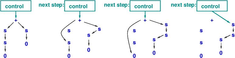
Modern object languages do work by constructing objects and calling their methods with arguments. Variable assignment is de-emphasized, hidden within objects. Can we dispense with assignment altogether? The object languages, Ocaml and Scala, try this.
The internet/web is a kind of "virtual machine" where there are no global variables --- most notably, there is no global clock "variable". Each node in the net sends/receives knowledge to/from other nodes, and "time" is relative. Do we need variables and assignments to program the internet? Modern languages move away from assignment.
Another reason why we might abandon assignment is because many programming errors arise due to updating cells in the wrong order or due to a race condition on updates on a shared cell. In multi-core processors, there are huge problems with synchronizing the updates saved in the cores' caches with the values saved in primary storage. These problems would disappear if we would prohibit updates to memory cells once the cells are initialized --- all variables should be declared as final (in Java) or readonly (in C#) or val (in Scala) --- one value only. It's a radical proposal, but it leads us to surprising solutions to traditional problems.
Fifty years ago, memory cells were expensive, storage had to be reused, and assignment was a form of memory management. Today, storage is cheap and there is no need to "destroy" "old" values. (For example, Gmail never deletes emails, even if you tell it to. Facebook keeps everything, too, alas.) The assignment statement has lost much of its importance. (What about assignments in loop bodies? It turns out we can do without loops as well --- we see how in this chapter.)
There is a paradigm of programming, the functional paradigm, that dispenses with traditional assignment --- once a name is initialized to a value, that value can never be updated. Examples of functional programming languages are Lisp, Scheme, ML, and Haskell. We study their principles in this chapter. Once you learn about these, you can move to modern object languages that de-emphasize or eliminate assignment, like Scala and Ocaml, and modern functional network languages, like Bloom/CALM.
We first look at a new virtual machine, one that has no assignment. Then we reexamine the heap virtual machine but restrict it so that all bindings made in namespaces are final (that is, once initialized, cannot be changed).
   +-----+
   | CPU | (controller)
   +-----+
      |
      V
+---------------+-+-+- ... +-+-+
| program codes | | |      | | |
+---------------+-+-+- ... +-+-+
                (data table saved in cells)
The program updates the data table's cells over and over until the
instructions are finished.
The von Neumann machine is based on a theoretical model known as
the Universal Turing machine, which looks much like the picture
above.
Tables (e.g., data bases) are certainly important,
but not all computations are table driven. Think about arithmetic!
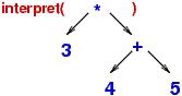
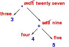
Here is a "program" --- (3 * (4 + 5)) --- and its computation:
(3 * (4 + 5)) = (3 * 9) = 27
Here,
computation rewrites the program until it can be rewritten no more.
There are no ``cells'' to update.
The rewriting rules for arithmetic can be stated in equation style,
using a formalism called a Post system.
When you were a child, you memorized this massive "Post system" of
equations for doing addition:
0 + 0 = 0
0 + 1 = 1      1 + 0 = 1
1 + 1 = 2      0 + 2 = 2      2 + 0 = 2
1 + 2 = 3      2 + 1 = 3      0 + 3 = 3    3 + 0 = 3
3 + 1 = 4      1 + 3 = 4      2 + 2 = 4    0 + 4 = 4     4 + 0 = 4
  and so on ...
If we represent
(nonnegative)
numbers in Base 1 format (e.g., 0 is 0, 1 is s0, 2 is ss0, 3 is sss0, etc.), then only four equations
are needed to define addition and multiplication:
===================================================

0 + N =  N                 (1)
sM + N =  M + sN           (2)

0 * N =  0                 (3)
sM * N =  N + (M * N)      (4)

===================================================
M and N are algebra-style variables, e.g.,
we compute 2 + 2 (that is, ss0 + ss0) like this:
   ss0 + ss0
              matches Rule (2), where  M is s0  and  N is ss0
=  s0 + sss0
              matches Rule (2), where  M is 0  and  N is sss0
=  0 + ssss0
              matches Rule (1), where  N is ssss0
=  ssss0
Next, we compute 3 * 2, that is, sss0 * ss0, like this:
   sss0 * ss0
=  ss0 + (ss0 * ss0)                by Rule (4)
=  ss0 + (ss0 + (s0 * ss0))         by Rule (4)
=  ss0 + (ss0 + (ss0 + (0 * ss0)))  by Rule (4)
=  ss0 + (ss0 + (ss0 + 0))          by Rule (3)
=  ... =  ss0 + (ss0 + ss0)         by Rules (1) and (2), like above
=  ... =  ss0 + ssss0               by Rules (1) and (2), like above
=  ... =  ssssss0                   by Rules (1) and (2), like above
You can imagine that we might wire the four equations into the ALU of
a hardware computer:
+----------------------------------+
| hard-wired equations for * and + | (ALU)
+----------------------------------+
      |
      V
+------------------------+
| arithmetic expression  | (storage)
+------------------------+
This rewriting machine repeatly scans the arithmetic expression, searching for a
phrase that can be rewritten by one of the equations for * and +.
There is no instruction counter, nor data cells.
(Indeed, a real-life ALU has the equations for base-2 addition and multiplication hard-wired into it! The wiring looks at the 1/0 patterns in the CPU's index registers and rewrites them. After all, electronic computers were first built for doing arithmetic!)
In the above "arithmetic machine,"
The arithmetic-expression part is better represented as an operator tree,
which is easy to traverse, match, and build:
Links are moved, nodes are constructed, and an answer is built.
Unneeded nodes remain as garbage, but these can be
erased by a garbage collector.
This layout will lead to a beautiful solution to storage sharing.
Based on the arithmetic example,
you can imagine a ``universal rewriting machine,''
which operates with user-defined equations and an expression:
  +-------------------------+
  | equation-rewrite engine | (ALU)
  +-------------------------+
      |            |
      V            V
+------------+-----------------+
| equations  | expression tree | (storage)
+------------+-----------------+
Now, the human can write down any equations at all --- a kind
of equation-computer program --- and insert them into the machine's
"equations" storage. The
machine will repeatedly match equations in the ''equations'' part
to subtrees in the ``expression tree'' part and do rewriting.
There is no sequential code, no instruction counter, no data cells ---
only equations and a tree that is constantly reconfigured.
This is a different paradigm than the Turing/von Neuman machine. It is called a Post system and it
has been proved to be "universal" --- as equally computationally powerful as
Turing machines and all other known computational mechanisms.
Physicists, chemists, mathematicians, etc., find the equation-rewrite machine to be a more natural model than the von Neumann/Turing machine. We must take this very seriously....
HISTORICAL NOTE: The first non-assembly programming language, Fortran, was invented so that physicists could write their programs as equations to be solved. John Backus, Fortran's inventor, built a compiler (the first compiler!) that mapped the equations into machine code for a von-Neumann machine. It was easier for Backus to use storage cells to hold the equations' "answers" than to emulate a virtual machine that did equational rewriting --- Backus had his hands full inventing parsing and machine translation! Incidentally, when Backus received the Turing Award in 1977, he made a speech disavowing assignment languages: Can Programming Be Liberated from the von Neumann Style? A Functional Style and Its Algebra of Programs (Comm. ACM, Vol 21-8, August 1978).
There is an even more exotic version of computational language for
rewriting, called the
lambda calculus (devised by Alonzo Church around 1920), where there is only one operator,
λ, and programs and data are coded just with it and algebra
variables. Here are some codings:
0 is   (λs(λz z))
1 is   (λs(λz (s z)))
2 is   (λs(λz (s (s z))))
     and so on

M + N  is  ((M plusOne) N)
      where   plusOne  is   (λn(λs(λz (s ((n s) z)))))

M * N  is  ((M +) N)
There is just one rewrite equation for λ:
((λx M) N) =  [N/x]M
   where  [N/x]M  is the replacement of all (free) occurrences of  x  by  N  in M
The lambda-calculus is equally computationally powerful to Post systems and
Turing/von Neuman machines.
We will examine it later in the chapter.
Now we are ready to learn the functional programming paradigm, which does computing as program rewriting.
But every spreadsheet program has an "undo" button, which lets the user backtrack (erase) the most recent update and recover the spreadsheet that existed before. How does the spreadsheet program implement the "undo"?
One answer is --- the spreadsheet table isn't updated by
assignment. Although
the user believes she inserted a new value into
a cell, the spreadsheet program retains both the cell's old value and its
new value. For example, if the spreadsheet is a vector,
   (pointer to the vector)
    |
    v
    0  1  2   ...    i ...
   +--+--+--+- ... -+--+- ...
   |a |b |c |       |n |
   +--+--+--+- ... -+--+- ...
and the user updates cell i with value m, then the
program builds this data structure, which chains the update
onto the front of the vector:
  (pointer to the vector)
   |
   v
   i       0  1  2   ...    i ...
  +--+    +--+--+--+- ... -+--+- ...
  |m |+-->|a |b |c |       |n |
  +--+    +--+--+--+- ... -+--+- ...
When the spreadsheet is searched for entry i, the pointer leads
us to value m. When the spreadsheet is searched for entry 2, the pointer leads
us to cell i and then to the other cells, where b is found.
When painted on the computer's display,
the data structure is painted to look like a vector
where m lives in cell i.
But since the data structure holds both the original value and the update, "undos"
are easily achieved (just reset the pointer!) --- the assignment implemented
by the spreadsheet program does not alter values already in storage.
(NOTE: maybe you expected this answer, which maintains a stack of
"undo" actions:
 0  1  2   ...    i ...
+--+--+--+- ... -+--+- ...
|a |b |c |       |m |
+--+--+--+- ... -+--+- ...

            +-----+-------+--(top)
undo stack: | ... | i = n |
            +-----+-------+--
Here, the old value of cell i is copied to a stack in case it needs to be
reinserted. We are lucky that it is easy to reverse the assignment,
i = m by executing i = n. But it is not always this easy --- see below.)
There is another, crucial advantage to the nondestructive implementation: if the spreadsheet/database is shared by multiple processes, each of which is doing its own search or computation on the database, all processes may proceed in parallel even while updates are being performed, because each process has a "pointer" to the instance of database it uses. This is common for a database shared through the Web. Of course, the answer computed by a process is correct for the database at the time it was accessed, that is, the answer must be time-stamped. Time stamps can be compared later and answers reconciled, if necessary (this is called "relaxed consistency") --- after all, there is no single global clock for the Web.
Here is a second example, where it is difficult, if not impossible, to reverse
changes.
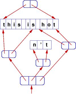
When you use a text editor to change a text file, you insert new text
within lines in the file. The changes you make are not
done immediately; they are patched onto the original lines in the file.
For example, we might start with this line of text
and insert n't in the middle. The text editor patches the insertion
onto the line somewhat like this:
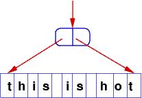
The text editor displays what looks like the altered text line,
but the original line is still there and the insertion can be "undone"
by changing the pointer back to its original value.
Only when the file of lines is written to disk are the changes traversed and copied to disk
as a sequence of characters.
The same approach is used for real-life data bases and any structure where there must be the ability to perform and undo complex updates.
Arithmetic is for playing ``number games.'' Many computing problems are ``data-structure games,'' where we assemble and disassemble data structures like stacks, queues, trees, and tables. We can do some of this already in Python:
>>> x = 2
>>> print x + 3   # use  x  in arithmetic
5
>>> print x
2                 # x  is unchanged, of course
>>> print 2 + 3   # for that matter, no need for  x...
5
>>> s = "abc"
>>> print s[1:] + s[0]           # use  s  in "string arithmetic"
bca
>>> print s
abc                              # s  is unchanged
>>> print "abc"[1:] + "abc"[0]   # really no need for  s
bca
>>> m = ["a", ["b","c"], []]
>>> print m[1:] + [m[0]]         # use  m  in "list arithmetic"
[['b', 'c'], [], 'a']
>>> print m
["a", ["b","c"], []]             # m  is unchanged
>>> ["a",["b","c"],[]][1:] + [ ["a",["b","c"],[]][0] ]  # no need for  m
[['b', 'c'], [], 'a']
MacCarthy wanted to train a computer to read, write, and think in terms of words and sentences, like a human does. (MacCarthy was a founder of Artificial Intelligence.) At the time, the only non-assembly programming languages available were Fortran (for numerical computation on vectors and matrices) and Cobol (for formatting and printing business documents). Neither would work for manipulating language.
MacCarthy viewed sentences as nested lists of phrases and words, and he wanted an "arithmetic language" for them. As a trained mathematician, MacCarthy knew that his "list arithmetic" could be extended by recurrence equations that would define repetitive patterns.
Here is a tiny language that resembles core Lisp or core ML:
===================================================

E: Expression
A: Atom (words)

E ::=  A  |  nil  | E1 :: E2  |  hd E  |  tl E |  ifnil E1 then E2 else E3
A ::= strings of letters

===================================================
"a" :: nil is a list of one element. (We can write this as ["a"] in Python and ML.)
"b" :: ("a" :: nil) is a two-element list, where "b" is first and "a" second. (We write this as ["b", "a"] in Python and ML.) :: is a kind of ``stack push.'' (In Python, we would simulate E1::E2 as [E1] + E2.)
A list of form, "a1" :: ("a2" :: (... :: ("an" :: nil) ...)) will be written as "a1"::"a2"::...::"an"::nil. (In Python and ML, the list is ["a1", "a2", ..., "an"].)
Lists can be nested and can be a mix of atoms and lists, e.g., nil::("b"::"c"::nil)::"d"::nil is a nested list (and it looks like [[], ["b", "c"],"d"] in Python).
In Lisp, :: is written cons (for ``construct'') e.g., (cons "b" (cons "a" nil)). For this reason, we read :: as "cons".
We will not do this often, but we can write, say, "a" :: "b", as well as nil :: "a". These structures are called dotted pairs, and they are like Python pairs (e.g., ("a", "b") and ([], "a")).
===================================================

hd (E1 :: E2)  =  E1                        (i)

tl (E1 :: E2)  =  E2                        (ii)

ifnil nil then E1 else E2  =  E1            (iii)

ifnil (E1 :: E2) then E3 else E4  =  E4     (iv)

===================================================
Note: some people add this equation, so that the conditional can test on atoms as well as lists:
===================================================

ifnil A then E1 else E2  =  E2              (v)

===================================================
The equations define
an ``arithmetic'' for lists.
Here's some arithmetic, calculated "inside out":
hd(tl ("a"::"b"::(tl ("c"::nil))))

= hd(tl ("a"::"b"::nil)))  # rule (ii)

= hd ("b"::nil)            # rule (ii)

= "b"                      # rule (i)
hd and tl are "searching" the list.
The above example can also be calculated "outside in":
hd(tl ("a"::"b"::(tl ("c"::nil))))

= hd("b"::(tl ("c"::nil)))  # rule (ii)

= "b"                       # rule (i)
This save us one rewriting step.
Here is a third example, using a nested list:
"a" :: (tl (hd (("b"::nil)::"c"::nil)))

= "a" :: (tl ("b" :: nil))      # rule (i)

= "a"::nil                      # rule (ii)
When an expression rewrites to its "answer form" (where no more rules can rewrite the expression), the answer form is called
the expression's normal form.
Here's another example:
ifnil ("a" :: nil)
  then  nil
  else  hd (tl ("b" :: "c" :: nil))

= hd (tl ("b" :: "c" :: nil))        # rule (iv)

= hd ("c" :: nil)  =  "c"            # rules (ii) and (i)
The order in which we use the equations does not matter
since there is no assignment nor sequencing.
The previous example could be worked like this:
ifnil ("a" :: nil)
  then  nil
  else  hd (tl ("b" :: "c" :: nil))

= ifnil ("a" :: nil)
    then  nil
    else hd ("c" :: nil)

= ifnil ("a" :: nil)
    then  nil
    else "c"

= "c"
We
get the same answer (normal form) with our equations, regardless of the order we apply them.
This is called the confluence or Noetherian property of a
rewriting system.
So far, our language doesn't look like much, but we can represent numbers with lists: the number, n, is the list, "s"::"s"::...::"s"::nil, where "s" is repeated n times. In a moment, we will write equations for computing addition, subtraction, etc. Further, we can represent a vector as a list, a matrix as a list of lists, a tree as a nested list, and so on.
Our core language with its semantics is "list algebra". In algebra class, we give names to numbers and to functions. Let's add these to the core language, applying Tennent's abstraction and parameterization principles.
Here is a first, modest extension: top-level definitions:
===================================================

P: Program               D: Declaration
E: Expression            I: Identifier
A: Atom (words)

P ::=  D* E
       where D* means zero or more D phrases

D::=  val I = E .  |  fun I ( I* ) = E .

E ::=  A  |  nil  | E1 :: E2  |  hd E  |  tl E
    |  ifnil E1 then E2 else E3  |  I  |  I ( E* )

A ::= strings of letters

===================================================
Here is an example and its computation:
val x = "a"::"b"::nil.
val y = x :: x.
fun second(L) = hd(tl L).
second(y)

second(y) = hd(tl y) # replace  second  by its body and insert its argument
= hd(tl (x :: x))    # replace  y  by its body
= hd x               # law (i):  hd(E1 :: E2) = E1
= hd("a"::"b"::nil)  # replace  x  by its body
= "a"                # law (i)
Here are functions for addition and multiplication on
base-1 numerals:
===================================================

fun add(M, N) = ifnil M then N
                        else add(tl M, ((hd M)::N)).

fun mult(M, N) = ifnil M then nil
                         else add(N, mult((tl M), N)).

val two = "s"::"s"::nil.
val three = "s"::two.

mult(three, two)

===================================================
The functions add and mult are recodings of the two Post
equations we saw at the start of the chapter.
This little program computes mult(three two) to 6 (more precisely, to
"s"::"s"::"s"::"s"::"s"::"s"::nil):
===================================================

mult(three, two)

= ifnil three then  nil
              else add(two, mult(tl three, two))
= ifnil "s"::two then  nil
              else add(two, mult(tl three, two))

= add(two, mult(tl three), two))
= add(two, mult(tl (s::two)), two))
= add(two, mult(two, two))

= add(two, ifnil two then  nil
                     else  add(two, mult(tl two, two)) )
= ...
= add(two, add(two, mult("s"::nil, two)) )
= ...
= add(two, add(two, add(two, mult(nil, two))))
= add(two, add(two, add(two, ifnil nil then nil
                             else add(two, mult((tl nil), two)))))

= add(two, add(two, add(two, nil)))

= add(two, add(two, ifnil two then nil
                    else add(tl two, ((hd two)::nil))))
= ...
= add(two, add(two, add("s"::nil, "s"::nil)))
= ...
= add(two, add(two, add(nil, "s"::"s"::nil))
= ...
= add(two, add(two, "s"::"s"::nil))
= ...
= add(two, "s"::"s"::"s"::"s"::nil)
= ...
=  "s"::"s"::"s"::"s"::"s"::"s"::nil

===================================================
The rewritings were performed largely "inside out", but there is no
required order since we are doing equational rewriting --- the final answer will always be the same.
The semantics of function call is copy-rule semantics --- replace the call by the function's body, binding arguments to parameters:
===================================================

I(E1, E2, ..., Em)  =  [Em/Im]...[E2/I2][E1/I1]E ,
                    if  fun I(I1, I2, ..., Im) = E

   where [E'/J]E  stands for the substitution of E'
   for all occurrences of identifer J in E

===================================================
(See the first simplification in the previous example: three replaced
M and two replaced N in the body of mult.)
Here is an example to think about:
val As = "a" :: As.
hd(tl(tl As))
The answer is "a":
hd(tl(tl As))
=  hd(tl(tl ("a"::As)))
=  hd(tl As)
=  hd(tl ("a"::As))
=  hd As
=  hd("a"::As)  =  "a"
As names a list that expands to as many "a"s as we would ever want. Indeed, that's exactly what happens in the functional programming language, Haskell.
To summarize, in the functional paradigm, a "program" is a "data structure", and computation is the rewriting of structure into a normal form.
Maybe baby arithmetic does not impress you. But think about a big database, designed as a nested tree or trie or table. Such a database can be coded as a nested list, with a pointer/handle to its entry point. Now think about a database query: a search function is called with (i) a handle to the huge, nested-list database and (ii) a query, itself coded as a nested list or even as a function. The search(database, query) function traverses the database and "disassembles" the query much in the same way that mult and add above traversed and disassembled its arguments. The search(database, query) call rewrites to the result of the query.
And at the very same time, other searches and even other updatees can be called, each receiving as a parameter the handle to the massive database. As stated in the first section of this chapter, the functional paradigm allows the calls to work in parallel, because the database is not destructively updated --- any updates are "patched onto" the database --- no data within the database is ever erased. We see how this is implemented later in the chapter.
===================================================

P: Program               D: Declaration
E: Expression            I: Identifier
A: Atom (words)

P ::=  D* E     where D* means zero or more D phrases

D::=  val I = E .  |  fun I ( E* ) = E2 .

E ::=  A  |  nil  | E1 :: E2  |  hd E  |  tl E
    |  ifnil E1 then E2 else E3  |  I  |  I ( E* )

A ::= strings of letters

===================================================
A function is declared with expressions, more precisely, with
expression patterns:
fun I(E*)= E2.
An expression pattern shows the form of argument that is allowed
to be given to a function. The pattern will contain identifiers
that "match" to the argument.
Here is a small example, which extracts the second element in a list:
fun second(M::N::L) = N.
We can call it like this:
second("a"::"b"::"c"::nil)
  = "b"   # "a" matches M,  "b" matches N,  "c"::nil matches L

second("a"::(tl ("b"::nil))::nil)
  =  tl ("b"::nil)  # "a" matches M,  tl ("b"::nil)  matches N,  nil matches L

second(tl ("a"::"b"::"c"::nil))   # cannot be called yet, doesn't match the pattern

second("a")  # cannot be called ever.  it's stuck --- an error
Functions with patterns can be defined in multiple clauses.
Here is a function that subtracts one, if possible, from
a base-1 numeral:
fun pred("s"::M) = M.
fun pred(nil) = nil.
This is a valid call: pred("s"::"s"::nil), which returns "s"::nil.
This is not yet a valid call: pred(tl ("s"::"s"::nil)).
Once tl ("s"::"s"::nil) computes to "s"::nil, then
pred can execute and return nil.
Finally, pred(nil) computes to nil.
Here is the earlier arithmetic example with its functions
coded with patterns.
===================================================

fun add(nil,    N)  =  N.                     // (1)
fun add("s"::M, N)  =  add(M, "s"::N).        // (2)

fun mult(nil,    N) =  nil.                   // (3)
fun mult("s"::M, N) =  add(N, mult(M, N)).    // (4)

val two = "s"::"s"::nil.
val three = "s"::two.

mult(three, two)

===================================================
A function call is rewritten to the body of that function declaration
whose patterns match the arguments of the call.
Here is the example, reworked. (It's shorter this time!)
mult(three, two)
=  mult("s"::two, two)                         // matches (4)
=  add(two, mult(two, two))
=  add(two, mult("s"::"s"::nil, two))          // matches (4)
=  add(two, add(two, mult("s"::nil, two))      // matches (4)
=  add(two, add(two, add(two, mult(nil, two))  // matches (3)
=  add(two, add(two, add(two, nil)))
=  add("s"::"s"::nil, add(two, add(two, nil))) // matches (2)
=  add("s"::nil, "s"::(add(two, add(two, nil))))
=  ...
=  "s"::"s"::(add(two, add(two, nil)))
=  ...
=  "s"::"s"::"s"::"s"::"s"::"s"::nil
Parameter patterns lets us code Post equations more faithfully.
A modern programming language lets you use parameter
patterns.
We'll use them a lot in the rest of the chapter.
NOTE: a standard restriction, for implementation efficiency, is that all the variables in a function's patterns are distinct. That is, fun add("s"::M, N) =... is allowed, but fun add("s"::M, M) =... is not. Also, patterns are often restricted to expressions with assembly operators only, e.g., fun add("s"::M, N) =... is allowed, but fun add((tl M), N) =... is not.
E: Expression     A: Atom

  E ::=  A  |  ( E1 E2 ... En )
  A ::=  nil  |  hd  |  tl  |  cons  |  ifnil  |  stringsOfLetters
The language syntax we use in this chapter is based on Standard ML, not Lisp, but you will see MacCarthy's ideas reappear in all the examples that follow.
The next sections develop these principles. You have a choice:
===================================================

D: Definition
E: Expression
A: Atom
I: Identifier

E ::=  A  |  nil  |  E1 :: E2  |  hd E  |  tl E
    |  ifnil E1 then E2 else E3  |  let D in E end  |  I

D ::=  val I = E

===================================================
The abstraction and qualification principles are at work here:
val I = E binds identifier I to expression E --- it is a kind of equation, added to the programming language.
Now, whenever we mention I, it means E and
can be substituted by E, equals for
equals. I is not a location in storage, it is a constant value.
(Java/C# let you declare a ``final variable'' that is
initialized and fixed forever, e.g., final double pi = 3.14159.)
We add one new rewriting equation to our semantics, which explains how to the val equation computes:
===================================================

let val I = E1 in E2 end  =  [ E1 / I ] E2

===================================================
where [ E1 / I ] E2 means that we substitute the phrase E1 for all
(free) occurrences of name I within phrase E2.
For example:
let val x = "a" in (x :: x) end = ["a"/x](x :: x) = ("a" :: "a")
Here is another example:
let val x = "a" :: nil  in
let val y = "b" :: x  in
x :: (tl y)
end end
This can compute as follows:
===================================================

let val x = "a" :: nil  in
let val y = "b" :: x  in
x :: (tl y) end end

= let val y = "b" :: ("a" :: nil) in
  ("a" :: nil) :: (tl y) end

= ("a" :: nil) :: (tl ("b" :: ("a" :: nil)))

= ("a" :: nil) :: ("a" :: nil)

===================================================
The answer displays as the list, [["a"], "a"], in Python.
The example can be worked in another order:
===================================================

let val x = "a" :: nil  in
let val y = "b" :: x  in
x :: (tl y) end  end

= let val x = "a" :: nil  in
  x :: (tl ("b" :: x) end

= let val x = "a" :: nil  in
  x :: x              end

= ("a" :: nil) :: ("a" :: nil)

===================================================
Sequencing does not matter when there are no assignments!
let definitions can be embedded,
like this:
tl (let x = nil in x :: (let y = "a" in y :: x end) end)
which computes to
===================================================

= tl (let x = nil in x :: ("a" :: x) end)

= tl (nil :: ("a" :: nil))

= "a" :: nil

===================================================
Here is a more delicate example, where we redefine x in nested
blocks. (This is similar
to writing a procedure that contains a local variable of the same
name as a global variable.)
===================================================

let val x = "a"  in
    let val y = x :: nil  in
        let val x = nil  in
           y :: x
        end
    end
end

===================================================
If we substitute carelessly, we get into trouble!
Say we substitute for y first and appear
to get
let val x = "a"  in
   let val x = nil  in
      (x :: nil) :: x
   end
end
This is incorrect --- it confuses the two definitions of x and
there is no way we will obtain the correct answer,
("a" :: nil) :: nil.
The example displays a famous problem that dogged
19th-century logicians. The solution is, when we substitute
for an identifier, we never allow a clash of two definitions ---
we must rename the inner definition, if necessary.
In the earlier example, if we substitute for y first, then
we must eliminate the clash between the two defined xs by renaming the
inner x:
===================================================

let val x = "a"  in
    let val y = x :: nil  in
        let val x' = nil  in
           y :: x'
        end
    end
end

===================================================
Now the substitution proceeds with no problem.
We can define substitutation and renaming precisely with equations.
The equations cover all possible cases of substitution and only the last
3 equations are interesting:
===================================================

let val I = E1 in E2 end  =  [ E1 / I ] E2

where

[ E0 / I ] A  =  A           # atoms are left alone

[ E0 / I ] nil  =  nil       # so is nil


[ E0 / I ] E1 :: E2  =  [ E0 / I ]E1 :: [ E0 / I ]E2    # substitute into both parts

[ E0 / I ] hd E  =  hd [ E0 / I ]E    # substitute into the subexpression...

[ E0 / I ] tl E  =  tl [ E0 / I ]E

[ E0 / I ] ifnil E1 then E2 else E3  =
    ifnil  [ E0 / I ]E1  then  [ E0 / I ]E2  else  [ E0 / I ]E3

[ E0 / I ] let D in E end  =  let  [ E0 / I ]D  in  [ E0 / I ]E  end


[ E0 / I ] I  =  E0     # replace  I

[ E0 / I ] I' =  I'     if  I' not= I   # don't alter a var different than I


[ E0 / I ] val I' = E   =   val I' = [ E0 / I ]E   if  I not= I' and  I' does not appear in  E0
       # that is, if there is no name clash


[ E0 / I ] val I = E   =   val I = E    # do nothing because  I is redefined here


[ E0 / I ] val I' = E   =   val I'' = [ E0 / I ][ I'' / I' ]E
       if  I not= I' and  I' appears in E0  and  I''  is a new name that does not appear in either  E0  or  E
            # if there is a name clash, rename  I'  to some new  I''

===================================================
The last equation makes clear that a name clash is repaired by inserting
an extra substitution to replace the name that clashes.
A machine based on equation rewriting can apply the above substitution laws without problem.
Exercise:
Build an interpreter --- a rewriting virtual machine --- that repeatedly applies these five equations:
===================================================

ifnil nil then E1 else E2  =  E1

ifnil (E1 :: E2) then E3 else E4  =  E4

hd (E1 :: E2)  =  E1

tl (E1 :: E2)  =  E2

let val I = E1 in E2 end =  [ E1 / I ] E2

===================================================
to an operator tree in the functional language until a normal form appears.
You have built the tree-rewriting machine shown in the Introduction section!
Such a machine would represent the program as an operator tree and
would repeatedly search the tree, top down, to find
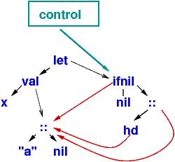
a subtree that matches an equation. For example, the program
let val x = "a" :: nil
in  ifnil x  then nil
             else (hd x) :: x
end
would compute like this:
Since this is a data structures language, computation is traversing
links between substructures and substitution (e.g.,
let val x = ... in ...) is moving links and not
copying code!
Here, the normal form (answer) is "a" :: ("a" :: nil).
This approach is used to implement the Haskell language.
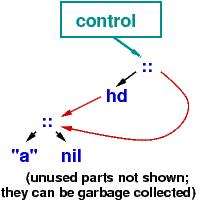
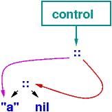
| Note: the first step above, the moving of all the links to represent the substitutions for x, can be expensive at runtime. The Haskell compiler will build this altered program "tree", upon which val operations execute much faster (at the price of an extra indirection step at variable lookup): |
|
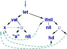
There is another approach that does not move links for substitution of
variables but builds a "normal-form tree" in the heap. This is the approach
used in Lisp, Scheme, and ML and what
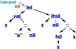
we will code in Python. Recall from Chapter 1
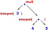
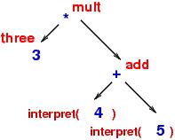
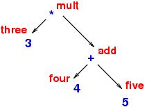
that function interpret traversed an expression
tree and computed its meaning by computing and combining the meanings of its
subtrees. In picture form, interpret computed somewhat like this:
The internal meanings are saved (somwhere!) in the same "shape" as the expression tree and are combined into the final answer, twenty seven.
This technique was first
invented for computing Lisp programs, and we now use it here.
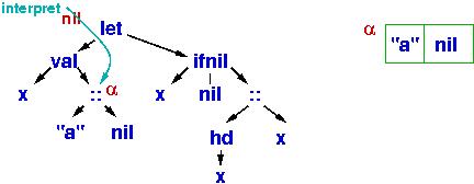
Our interpreter will traverse the operator tree, and when it computes the meaning of a subtree, it constructs the subtree's meaning in the heap in the form of two-celled objects, called cons cells. Each let subtree constructs a namespace. Once an object is constructed in heap storage, it is never altered. This allows massive, natural, sharing of data structures and eliminates sequencing, sharing, and race errors.
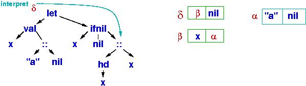
Here is the program at the beginning of this section:
(The nil subscript is the handle to the namespace that is used for
name lookups. At the beginning, no names are defined.)
Starting at the tree's root,
the interpreter must compute the value that will be named x, so
it descends leftwards:
The value is just
the subtree,
"a" :: nil, so the interpreter creates a cons cell in the heap,
and the handle of that cons cell, α, is the meaning of "a" :: nil.
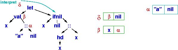
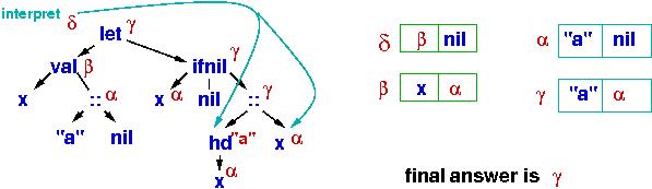
Next,
x binds to α in a new cons cell, β, and there is a binding list ("namespace"), δ, which points to the binding. The interpret function uses δ to
interpret the meaning of the subtree rooted by ifnil:
The test part of ifnil consults δ (then β) to learn that x's
value is α and not equal to nil. So, the else-arm is traversed:
Some work is needed to
compute the meaning of (hd x)::x --- x is looked up twice, then there
is a
head operation, and a cons cell is built to represent the final
answer:
The answer is handle γ, which prints as "a" :: ("a" :: nil).
Throughout the computation, α is used in multiple places
to represent the structure, "a" :: nil. The sharing is safe because
α's cons cell is never updated after it is first constructed.
For that matter, once constructed in the heap, no cons cell is ever changed.
Here is the Python-coded syntax of operator trees; it closely matches
the source syntax:
===================================================

ETREE ::=  ATOM  |  ["nil"]  |  ["cons", ETREE, ETREE] |  ["head", ETREE]
        |  ["tail", ETREE]  |  ["ifnil", ETREE1, ETREE2, ETREE3]
        |  ["let", DLIST, ETREE]  |  ["ref", ID]

DLIST ::=  [  [ID, ETREE]+ ]
        that is, a list of one or more  [ID, ETREE]  pairs

ATOM  ::=  a string of letters
ID    ::=  a string of letters, not including keywords

===================================================
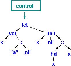
For example, the expression,
let val x = "abc" :: nil
    val y = ifnil x then nil else hd x
in
    y :: x
end
has this operator tree:
["let", [["x", ["cons", "abc", ["nil"]]],
         ["y", ["ifnil", ["ref", "x"],
                         ["nil"],
                         ["head", ["ref", "x"]] ]]],
        ["cons", ["ref", "x"], ["ref", "y"]]]
Here is the Python code for the functional language's interpreter:
===================================================

"""Interpreter for functional language with  cons  and  simple let.

Here is the syntax of operator trees interpreted:

ETREE ::=  ATOM  |  ["nil"]  |  ["cons", ETREE, ETREE] |  ["head", ETREE]
        |  ["tail", ETREE]  |  ["ifnil", ETREE1, ETREE2, ETREE3]
        |  ["let", DLIST, ETREE]  |  ["ref", ID]

DLIST ::=  [  [ID, ETREE]+ ]
        that is, a list of one or more  [ID, ETREE]  pairs

ATOM  ::=  a string of letters
ID    ::=  a string of letters, not including keywords

"""

### HEAP:

heap = {}
heap_count = 0  # how many objects stored in the heap

"""The program's heap --- a dictionary that maps handles
                          to namespace or cons-pair objects.

      heap : { (HANDLE : NAMESPACE or CONSPAIR)+ }
        where
         HANDLE = a string of digits
         NAMESPACE = {IDENTIFIER : DENOTABLE} + {"parentns" : HANDLE or "nil"}
            that is, each namespace must have a "parentns" field
         CONSPAIR = (DENOTABLE, DENOTABLE)
         DENOTABLE = HANDLE or ATOM or "nil"
         ATOM = string of letters

   Example:
     heap = { "0": {"w": "nil", "x": "ab", "parentns": "nil"},
              "1": {"z":"2", "parentns":"0"},
              "2": ("ab","nil"),
              "3": {"y": "4",  "parentns":"1"},
              "4": ("2","2")
            }
     heap_count = 5
        is an example heap, where handles "0","1","3"  name  namespaces
        which hold definitions for  w,x,z,y,  due to  let  expressions.
        Handles "2" and "4" name cons-cells that are constructed due to
        a use of  cons.
        This example heap might have been constructed by this expression:
         let val w = nil
             val x = "ab" in
         let z = x :: w in
         let y = z :: z in
          ...

       The values computed are  w = [],  x = "ab",  z = ["ab"], y = [["ab"], "ab"]
"""

### MAINTENANCE FUNCTIONS FOR THE  heap:

def isHandle(v) :
    """checks if  v  is a legal handle into the heap"""
    return isinstance(v, str) and v.isdigit() and  int(v) < heap_count


def allocate(value) :
    """places  value  into the heap with a new handle
       param:  value - a namespace or a pair
       returns the handle of the newly saved value
    """
    global heap_count
    newloc = str(heap_count)
    heap[newloc] =  value
    heap_count = heap_count + 1
    return newloc


def deref(handle):
    """ looks up a value stored in the heap: returns  heap[handle]"""
    return heap[handle]


### MAINTENANCE FUNCTIONS FOR NAMESPACES:


def lookupNS(handle, name) :
    """looks up the value of  name  in the namespace named by  handle
       If  name  isn't found, looks in the  parentns and keeps looking....
       params: a handle and an identifier
       returns: the first value labelled by  name  in the chain of namespaces
    """
    if isHandle(handle):
        ns = deref(handle)
        if not isinstance(ns, dict):
            crash("handle does not name a namespace")
        else :
            if name in ns :
                ans = ns[name]
            else :   # name not in the most local ns, so look in parent:
                ans = lookupNS(ns["parentns"], name)
    else :
        crash("invalid handle: " + name + " not found")
    return ans


def storeNS(handle, name, value) :
    """stores  name:value  into the namespace saved at  heap[handle]
    """
    if isHandle(handle):
        ns = deref(handle)
        if not isinstance(ns, dict):
            crash("handle does not name a namespace")
        else :
            if name in ns :
                crash("cannot redefine a bound name in the current scope")
            else :
                ns[name] = value


### INTERPRETER FUNCTIONS:


def evalPGM(tree) :
    """interprets a complete program
       pre: tree is an ETREE
       post: final values are deposited in heap
    """
    global heap, heap_count
    # initialize heap and ns:
    heap = {}
    heap_count = 0

    ans = evalETREE(tree, "nil")
    print "final answer =", ans
    print "pretty printed answer =", prettyprint(ans)
    print "final heap ="
    print  heap

    raw_input("Press Enter key to terminate")


def evalETREE(etree, ns) :
    """evalETREE computes the meaning of an expression operator tree.

      ETREE ::=  ATOM  |  ["nil"]  |  ["cons", ETREE, ETREE] |  ["head", ETREE]
        |  ["tail", ETREE]  |  ["ifnil", ETREE1, ETREE2, ETREE3]
        |  ["let", DLIST, ETREE]  |  ["ref", ID]

       post: updates the heap as needed and returns the  etree's value,
    """

    def getConspair(h):
        """dereferences handle  h  and returns the conspair object stored
           in the heap at  h
        """
        if isHandle(h):
            ob = deref(h)
            if isinstance(ob, tuple):  # a pair object ?
                ans = ob
            else :
                crash("value is not a cons pair")
        else :
            crash("value is not a handle")
        return ans


    ans = "error"
    if isinstance(etree, str) :  #  ATOM
        ans = etree
    else :
        op = etree[0]
        if op == "nil" :
            ans = op

        elif op == "cons" :
            arg1 = evalETREE(etree[1], ns)
            arg2 = evalETREE(etree[2], ns)
            ans = allocate((arg1,arg2))   # store new conspair in heap

        elif op == "head" :
            arg = evalETREE(etree[1], ns)
            ans, tail = getConspair(arg)

        elif op == "tail" :
            arg = evalETREE(etree[1], ns)
            head, ans = getConspair(arg)

        elif op == "ifnil" :
            arg1 = evalETREE(etree[1], ns)
            if arg1 == "nil" :
                ans = evalETREE(etree[2], ns)
            else :
                ans = evalETREE(etree[3], ns)

        elif op == "let" :
            newns = evalDLIST(etree[1], ns)  # make new ns of new definitions
            ans = evalETREE(etree[2], newns)  # use new ns to eval ETREE
            # at this point,  newns  isn't used any more, so forget it!

        elif op == "ref" :
            ans = lookupNS(ns, etree[1])

        else :  crash("invalid expression form")
    return ans


def evalDLIST(dtree, ns) :
    """computes the meaning of a sequence of new definitions and stores
       the  ID, meaning  bindings in a new namespace
           DTREE ::=  [ [ID, ETREE]+ ]
       returns a handle to the new namespace
    """
    newns = allocate({"parentns": ns})  # create the new ns in the heap
    for bindingpair in dtree :  # add all the new bindings to the new ns
        name = bindingpair[0]
        expr = bindingpair[1]
        value = evalETREE(expr, newns)
        storeNS(newns, name, value)
    return newns


def crash(message) :
    """pre: message is a string
       post: message is printed and interpreter stopped
    """
    print message + "! crash! ns=", ns, "heap=", heap
    raise Exception   # stops the interpreter


def prettyprint(value):
    if isHandle(value):
        v = deref(value)
        if isinstance(v, tuple):
           ans = "(cons " + prettyprint(v[0]) + " " + prettyprint(v[1]) +")"
        else :
           ans = "HANDLE TO DICTIONARY AT " + v
    else :
        ans = value
    return ans

===================================================
Install the above code and run it with Python.
Try at least these test cases:
evalPGM( ["cons", "abc", ["nil"]] )

evalPGM( ["head", ["cons", "abc", ["nil"]]] )

evalPGM( ["ifnil", ["nil"], ["head", ["cons", "abc", ["nil"]]], "def"] )

evalPGM( ["let", [["x", "abc"]], ["cons", ["ref", "x"], ["nil"]]] )

evalPGM( ["let", [["x", ["cons", "abc", ["nil"]]]],
                 ["cons", ["ref", "x"], ["ref", "x"]]])

evalPGM( ["let", [["x", ["cons", "abc", ["nil"]]], ["y", "nil"]],
                 ["cons", ["ref", "x"], ["ref", "y"]]] )
Study the heap layouts as well as the answers computed for each case.
IMPORTANT:: There is no activation stack in the interpreter! Instead, each interpretTREE function is parameterized on the handle of the namespace it should use for doing variable lookups. This technique accomplishes the same work of an activation stack --- the stack is ``threaded'' through the sequence of function calls.
IMPORTANT IMPORTANT: The interpreter is not an equation-rewriting machine, but its evalETREE function has coded in its logic the strategy of applying the rewriting equations, working from left-to-right, inside-out, upon the input expression.
IMPORTANT3: Perhaps you noticed that there is only one destructive assignment command in the entire interpreter: heap_count = heap_count + 1, which is used to generate new handles! All the other assignments are like ML let val namings --- once a name is given a value, the name is never reassigned. It is easy to perform functional-programming style in scripting languages, because you can use their dynamic lists and dictionaries!
Definitions can be parameterized;
the result are functions:
===================================================

E ::=  ... |  let D in E end  |  I  |  I ( E,* )
D ::=  val I = E  |  fun I1 ( I2,* ) = E  |  D1 D2

===================================================
where E,* means zero or more expressions, separated by commas
and I,* means zero or more identifiers, separated by commas.
When a function is defined, its code
is saved. When the function is called, its arguments
bind to its parameters, and the function's code evaluates.
Here is a small example:
===================================================

let fun second(list) = let val rest = tl list
                       in  hd rest
in
second(tl("a" :: ("b" :: ( "c" :: nil))))

===================================================
The argument binds
to the parameter name when the function is called.
The equational rewriting might go like this:
===================================================

second(tl("a" :: ("b" :: ( "c" :: nil))))

= second("b" :: ( "c" :: nil))

= let val list = "b" :: ( "c" :: nil) in   # bind the arg to the param
  let val rest = tl list in
  hd rest

= let val rest = tl("b" :: ( "c" :: nil)) in
  hd rest

= let val rest = "c" :: nil in
  hd rest

= hd ("c" :: nil)

= "c"

===================================================
But since there are no assignments, we can be "lazy" and delay the
rewriting of the argument, like this:
===================================================

second(tl("a" :: ("b" :: ("c" :: nil))))

= let val list = tl("a" :: ("b" :: ("c" :: nil))) in   # bind the arg to the param
  let val rest = tl list in
  hd rest

= let val rest = tl( tl("a" :: ("b" :: ("c" :: nil)))) in
  hd rest

= hd (tl(tl("a" :: ("b" :: ("c" :: nil)))))

= ... = "c"

===================================================
In the end, the answer is the same.
===================================================

let val x = tl("b" :: "a" :: nil)  in      # compute x's argument first
    let val y = (hd x) :: x  in
        tl y
    end
end

=  let val x = "a" :: nil  in             # now substitute for x
       let val y = (hd x) :: x  in
           tl y
       end
   end

= let val y = (hd ("a" :: nil)) :: ("a" :: nil) in
      tl y
  end

= let val y = "a" :: "a" :: nil  in
      tl y
  end

= tl ("a" :: "a" :: nil)  =  "a" :: nil

===================================================
Lazy evaluation is "argument last" evaluation, where the substitution rule is applied before the named argument is computed to its answer.
Here is the previous example, repeated in lazy evaluation:
===================================================

let val x = tl("b" :: "a" :: nil)  in
    let val y = (hd x) :: x  in
        tl y
    end
end

=  let val y = (hd tl("b" :: "a" :: nil)) :: tl("b" :: "a" :: nil)  in
       tl y
   end

= tl ((hd tl("b" :: "a" :: nil)) :: tl("b" :: "a" :: nil))

= tl("b" :: "a" :: nil)  =  "a" :: nil

===================================================
Sometimes, lazy evaluation will discover an answer faster than eager evaluation.
Also, there is a clever implementation of lazy evaluation based on moving
links in an operator tree; it was presented earlier.
The ML language uses eager evaluation, partly because it has a read operation, which lets a user supply input, and also because it uses an implementation
based on the interpreter design pattern seen in the earlier chapters.
Also, eager evaluation computes in a simpler way when names are redefined.
Consider the eager evaluation of
===================================================

let val x = "a" in
    let val y = x :: nil in
        let val x = "b" in
            x :: y
        end
    end
end

= let val y =  "a" :: nil in
      let val x = "b" in
          x :: y
      end
    end

= let val x = "b" in            =  "b" :: "a" :: nil
          x :: ("a" :: nil)
      end

===================================================
Lazy evaluation is more subtle, because it does not demand that one
do substitutions in any specific ordering. What happens if we substitute
for y first in the above example?
===================================================

let val x = "a" in
    let val y = x :: nil in
        let val x = "b" in
            x :: y
        end
    end
end

= let val x = "a" in
      let val x2 = "b" in    # we must rename the inner  x  to  x2 !
          x2 :: (x ::nil)
      end
  end

= let val x = "a" in      =  "b" :: "a" :: nil
      "b" :: x :: nil
  end

===================================================
Humans sometime forget to
rename the inner x to x2; computers implement exactly the substitution
laws that are listed in the earlier section,
Naming: Expression abstracts and the substitution law,
and they do it correctly.
Two sections ago, when we calcuated the function call, second(tl("a" :: ("b" :: ( "c" :: nil)))), we did not rewrite the function call in precisely the correct style --- we should substitute the code for second into the position where second is referenced. Let's reformulate this properly.
First,
the definition,
fun second(list) = let val rest = tl list
                   in  hd rest  end
can be written as an ordinary val-definition, by moving
the parameter name to the right of the equals sign:
val second = (list) let val rest = tl list
                    in  hd rest end
It is a tradition to place the word, lambda, in front of the
parameter name, (list), so that the reader can identify it clearly:
===================================================

val second = lambda (list) let val rest = tl list
                           in  hd rest end

===================================================
second is the same function, just formatted a little differently.
Now it is clear that second is the name
of the function code,
lambda (list) let val rest = tl list in hd rest end.
This construction is called a lambda abstraction or an anonymous function. Java, C#, Python, Ruby, etc., let you write lambda abstractions. (In C#, the lambda abstraction is called a delegate and has a much wordier definition.)
IMPORTANT: in ML, the lambda abstraction is coded with fn .. => ..,
for example,
val second =  fn list => let val rest = tl list  in
                             hd rest
                         end
The lambda expression comes with this semantic equation, which is a variant
of the one we use for let:
===================================================

(lambda (I) E1) E2  =  [ E2 / I ] E1

===================================================
The equation defines the semantics of function call, that is, binding
an argument to a function's parameter name so that the function's body
can execute.
Let's rework the example of second with the lambda abstraction:
let val second = lambda (list) let val rest = tl list in
                                   hd rest end
    in  second(tl("a" :: ("b" :: ( "c" :: nil))))
end
We substitute for second and then bind the argument to the parameter:
= (lambda (list) let val rest = tl list in
                     hd rest end           )(tl("a" :: ("b" :: ( "c" :: nil)))

= let val rest = tl(tl("a" :: ("b" :: ( "c" :: nil)))) in
      hd rest
  end

= hd(tl(tl("a" :: ("b" :: ( "c" :: nil)))))

= ... = "c"
The expression, lambda (list) .., is the function code, divorced
from its name. We copied the function code into the position where
the function is called. This is how substitution is
supposed to work: you replace a name by the value it names.
Using the new equation, for lambda, we bind the argument to its
parameter name, and
everything works smoothly.
Here is the ``minimal form'' of our functional language:
===================================================

E ::=  ...  |  let D in E end  |  I  |  E1 (E2,*)  |  (lambda (I,*) E)
    where  (P,*)  means zero or more  P  phrases, separated by commas
D ::=  val I = E

===================================================
A function body, lambda (I,*) E, is an expression,
just like nil or E1 :: E2, because it can appear as part of
val I = E or even anonymously within
an expression, e.g.,
"a" :: (lambda (x) x :: x)(nil)

=  "a" :: (nil :: nil)
The nameless function is
called ``lambda abstraction'' because it is a kind of
abstract, a naming device, for the parameter.
The lambda abstraction has a long, rich history, extending to the
debates in 19th-century philosophy that let to the development
of modern set theory and predicate logic. It also happens to be
quite useful for computation!
We can go further.
If we claim that let val I = E1 in E2 is just a "macro" for
(lambda (I) E2)(E1), then our language is just
===================================================

E ::=  I  |  E1 E2  |  (lambda (I) E)

===================================================
We can get by with just one parameter per function, because
(lambda (p1, p2, ..., pm) E) is just a "macro" for
(lambda (p1) (lambda (p2) ... (lambda (pm) E) ...)).
This minimal language is called the lambda calculus.
It has only one computation law, the law for binding an argument to
a lambda abstraction, called the β-rule:
===================================================

β:    (lambda (I) E1) E2  =   [E2 / I ] E1

===================================================
Notice that there are no longer primitive values. like atoms or ints --- everything is a lambda abstraction --- a "function".
The lambda calculus is a language of functions that compute upon functions and compute answers that are functions.
The lambda calculus was invented by a mathematician-logician, Alonzo Church,
around 1910, to study the uses of namings in mathematical formulas and mathematical proofs. Church and one of his students, Steven Cole Kleene, saw how to code
base-1 arithmetic in the language,
Here is how they coded numbers as "functions":
===================================================

0  is  (lambda (s) (lambda (z) z))
1  is  (lambda (s) (lambda (z) s z))
2  is  (lambda (s) (lambda (z) s(s z)))
3  is  (lambda (s) (lambda (z) s(s(s z))))
   . . .

===================================================
There is an important reason for this coding --- an int, like 2, is now a "function" that "does s two times to z."
This coding comes from earlier work by Kurt Goedel, who formalized algorithms
for integers in logic. Goedel showed that many standard operations on ints
are expressed in this equational format:
   f (0)   = someAnswer
|  f (n+1) = doSomethingTo(f(n))
This style is called simple recursion.
The pattern works like this:
f(2) =  doSomethingTo(f(1))
     =  doSomethingTo(doSomethingTo(f(0))
     =  doSomethingTo(doSomethingTo(someAnswer))
Church and Kleene turned simple recursion "inside out": the function call,
f(m), is written in lambda calculus as
m doSomethingTo someAnswer
For example, f(2) looks like this in lambda calculus:
(lambda (s) (lambda (z) s(s z))) doSomethingTo someAnswer

= (lambda (z) doSomethingTo(doSomethingTo z)) someAnswer

= doSomethingTo(doSomethingTo(someAnswer))
List data structures can be coded
like this, using the "argument first" style that was used with numbers:
===================================================

E1 :: E2        is   (lambda (b) (b E1) E2)

hd E            is   E (lambda (h) (lambda (t) h))

tl E            is   E (lambda (h) (lambda (t) t))

nil             is   (lambda (b) (lambda (th) (lambda (el) th)))

ifnil E1 E2 E3  is   ( (E1  (lambda (h) (lambda (t) (lambda (th) (lambda (el) el)))) ) E2 )  E3

===================================================
These codings are
hard for a human to read, but a machine likes them just fine!
Kleene used these codings to express Goedel's
primitive-recursive functions, which have this equational format:
   f (m, 0)     =  someAnswer using m
|  f (m, n+1)   =  doSomethingTo(m, n, f(m, n))
Finally, Kleene defined an "unfolding operator",
Y = (lambda (f) (lambda (x) f(x x))(lambda (x) f (x x))),
that he used to
compute all possible forms of recursions (the general-recursive functions) and showed that these expressed all the algorithms that can be done on a Turing machine, or for that matter, on any computing machine.
Another of Church's students, Haskell Curry, saw that these lambda expressions,
I =  (lambda (x) x)
K =  (lambda (x) (lambda (y) x))
S =  (lambda (f) (lambda (g) (lambda (x) (f x)(g x))))
were special, because all possible lambda expressions could be recoded
using just these three "machine operations" (combinators),
S, K, I. (This approach is used to implement the OCAML programming
language!)
Research on the lambda calculus showed that a complete computational system could be built on the principles of rewriting, without destructive assignment. John MacCarthy was (somewhat!) aware of this work when he developed and implemented the first functional language, Lisp, in the late 1950s.
Perhaps this material seems esoteric, but the designers of Smalltalk, the first object-oriented language, modelled Smalltalk after the lambda-calculus --- in Smalltalk, all values, even numbers, are objects that can be called ("sent messages") and can return answers.
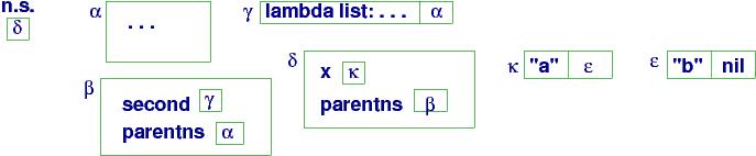
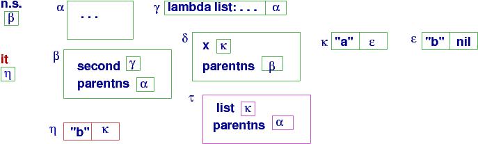
As before, a closure object is a pair, consisting of function-code-plus-parent-namespace-pointer. A couple of pictures will make this clear.
For this sample program:
===================================================

 . . .
let val second = lambda (list) hd (tl list)
in  let val x = "a" :: ("b" :: nil)
    in  second(x) :: x
    end
end

===================================================
The heap layout at the point where second is called
looks like this:
second's value, saved in namespace β, is the closure object
at handle γ. The closure remembers the code for the function
along with a link to its global names.
When second is called, namespace τ is created to hold its
parameter, list:
Once second returns its answer, "b" (because the tail of cons cell
κ is ε, and the head of its cons cell is "b"),
the current namespace reverts to δ, which lets us compute the
answer, the handle to a cons cell that holds "b" and κ:
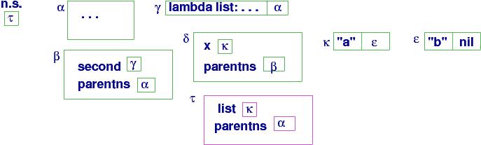
The answer is called it in ML. Here, it is the handle to a list.
It is easy to recode the interpreter in the earlier section to handle
this form of call. Note again that we don't require an activation
stack --- we parameterize the interpretTREE functions on the handle
of the current namespace used for lookups. That's it.
val f = fn n => if n = 0 then  1
                         else  n * f(n-1)
we will receive an error message stating that ''f is unbound'' (not defined).
The diagrams with the closure objects show why.
ML uses a special operator, rec, that we use when we want the environment handle saved in a named closure to refer to the environment holding
the very name being defined, that is, when we want recursion/self-reference.
Here's how it looks in ML:
val rec f = fn n => if n = 0 then  1
                             else  n * f(n-1)
These keywords might be interesting for theoretical reasons, but in practice,
the long-winded definition of f is stated in ML as merely,
fun f n = if n = 0 then  1
                   else  n * f(n-1)
The keyword, fun, means val rec .. = .. => ...
And we can do even better --- see the next section.
How many different ways can you shuffle a deck of, say, 5 cards?
The answer is a repeated multiplication:
fac(n) = 1 * 2 * 3 * ...up to... * n
So, fac(5) = 120, there are 120 distinct shuffles.
You have probably coded fac with a loop that
does the repeated multiplications.
But look at the pattern of nested multiplications inside the answer to fac(5):
fac(5) = 120 = (((1 * 2) * 3) * 4) * 5
We see that fac(5) = fac(4) * 5, and fac(4) = fac(3) * 4, and so on.
This nesting pattern is a recurrence,
and every computing person
knows that factorial is defined by
these recurrence equations:
===================================================

fac(0) = 1
fac(n) = n * fac(n-1),   for n > 0

===================================================
Most repetitive solutions are recurrences.
In the ML language, we use the two equations above to
compute factorial. Here is a calculation, like ML does:
fac(5) =  5 * fac(4)
       =  5 * 4 * fac(3)
       =  5 * 4 * 3 * fac(2)
       =  ...  =  5 * 4 * 3 * 2 * 1 * 1 =  120
The repeated multiplication is in a "counting-down" style, like a
loop does when it counts downwards from 5 to 0.
In older programming languages, we code fac
with if, like this:
fac(n) = if n = 0
         then 1
         else n * fac(n-1)
e.g.,
fac(3) =  if 3 = 0 then 1 else 3 * fac(3-1)
       =  3 * fac(3-1)
       =  3 * fac(2)

       =  3 * (if 2 = 0 then 1 else 2 * fac(2-1))
       =  3 * (2 * fac(2-1))
       =  3 * (2 * fac(1))

       =  ...
       =  3 * (2 * (1 * 1))  =  6
Here is an example that shows the power of recurrences.
Say that we want a list of all the values of factorial up to some limit point.
For example, faclist(6) = [720, 120, 24, 6, 2, 1, 1], which is
[fac(6), fac(5), ..., fac(0)].
We can write some loops to do this, but here is a smart solution in ML that
uses recurrence equations:
===================================================

faclist 0 = [1]
faclist n = let val subanswer = faclist (n-1)
            in  (n * (hd subanswer)) :: subanswer
            end

===================================================
For example,
faclist 5 = [120, 24, 6, 2, 1, 1],
but since fac(6) = 6 * fac(5), we can save a lot of time and
compute faclist 6 as (6 * (hd (faclist 5))) :: faclist 5!
The computation would unfold like this:
===================================================

faclist 6 = let val subanswer = faclist (6-1)
            in  (6 * (hd subanswer)) :: subanswer

          = let val subanswer = faclist 5
            in  (6 * (hd subanswer)) :: subanswer

          = ... many steps to compute  faclist 5  to the subanswer, [120, ..., 1] ...

          = let val subanswer = [120, ..., 1]
            in  (6 * (hd subanswer)) :: subanswer

          = (6 * (hd [120, ..., 1])) :: [120, ..., 1]

          = (6 * 120) :: [120, ..., 1]

          = 720 :: [120, ..., 1]  =  [720, 120, ..., 1]

===================================================
The omitted steps for the call, faclist 5, can be computed, just like above,
and you will see that faclist 5 rewrites to a call to faclist 4. And so on!
Just like the calculation of fac, there is a repeated calculation that "counts down" to 0. The final answer is assembled from the subanswers.
The rewriting semantics almost feels like there is a loop that is "running backwards"
from its "exit" to its "entry". But the computation is real and is correct!
One huge advantage of the equation format is that specifications and correctness
proofs are much much simpler than with loops.
Here is the specification and
correctness proof for faclist:
===================================================

(* faclist computes a list of factorials
      precondition: argument n >= 0
      postcondition: returns  [fac(n), fac(n-1), ...down to..., fac(0)]
*)
faclist 0 = [1]   (* proof of postcondition:  faclist 0 == [1] == [fac 0]   *)

faclist n = let val subanswer = faclist (n-1)
                  (* assert:  subanswer == [fac(n-1), ...down to..., fac(0)] *)
            in
            (n * (hd subanswer)) :: subanswer
                  (* proof:  faclist n == (n*fac(n-1)) :: [fac(n-1),...down to...,fac(0)]
                                       == (fac n) :: [fac(n-1),...down to...,fac(0)]
                                       == [fac(n), fac(n-1),...down to...,fac(0)]   *)
            end

===================================================
The above, smart definition computes the same answers as does this slower, naive, but also correct one:
faclist 0 = [fac 0]
faclist n = (fac n) :: faclist (n-1)
How would you code these computations as loops? How would you prove the loops
are correct?
Perhaps we want the list of numbers produced by faclist in ascending order. We reverse a list in ML
like this, using recursion to build the answer in
stages:
===================================================

(* reverse reverses the elements in a list.
   param: ns - a list, e.g, ["c","b","a"]
   returns: a list that holds the items of ns in reverse order, e.g., ["a","b","c"]
*)
fun reverse nil = []
|   reverse (x :: xs) =  (reverse xs) @ [x]   (* in ML,  @  means list append *)

===================================================
So, reverse(faclist 4) computes to [1,1,2,6,24]. We can calculate this:
===================================================

reverse [24, 6, 2, 1, 1] =  (reverse [6,2,1,1]) @ [24]
                  =  ((reverse [2,1,1]) @ [6]) @ [24]
                  =  (reverse [1,1]) @ [2] @ [6] @ [24]
                  =  ...
                  =  [] @ [1] @ [1] @ [2] @ [4] @ [8]
                  =  [1,1,2,6,24]

===================================================
The recursion was done with the tail of the argument list, that is, with a list that is one smaller than the original argument. In this way, we ``count down'' (disassemble) the list down to an empty one, which stops the recursions.
People who like loops often write this variant of list
reverse. The second parameter is called an accumulator, because
it accumulates the answer in stages:
===================================================

(* reverseloop(ns, ans)  reverses the items in list  ns  and appends them
    to the end of  ans.
   precondition:  both  ns  and  ans  are lists.
   postcondition: returns a list that holds the elements of  ans  followed by
    the elements of  ns  in reverse order.
   To use the function to reverse a list,  L,  do this:  reverseloop(L, []).
*)
fun reverseloop(nil, ans) = ans
|   reverseloop(n::ns, ans) = reverseloop(ns, n :: ans)

===================================================
This should remind you of the Post equations at the beginning of the chapter that
defined addition and multiplication on base-1 numerals.
We can easily write a function that searches
a list for a value:
===================================================

(* member(v, xs)  searches list  xs  to see if  v  is a member in it.
   params:  v - a value;  xs - a list of values
   returns: true exactly when  v  is found in  xs
*)
fun member(v, nil) = false
|   member(v, (w::rest)) = if v = w  then true
                           else member(v, rest)

===================================================
The function searches the list from front to back.
Recursion with parameters can substitute for assignment and iteration.
This loop,
x = 0
while x < 100 :
    print x
    x = x + 1
end
uses destructive assignment to count to 100.
But we can count with a function and a parameter:
In ML, we write
let fun printloop(x) = if x < 100
                       then (print(Int.toString(x)); print("\n");
                             printloop(x+1))   (* keep counting *)
                       else nil      (* else done -- do nothing *)
in printloop(0)
end
(ML has a print expression that prints a string and returns nil
as its answer. Use it with parens and a ; operator that sequences one expression
followed by another.)
Here is a useful ML function that reads a sequence
of text lines from the keyboard and assembles the lines into a list.
The function reads one line and restarts itself to
read more lines. It quits when it sees a "!":
===================================================

(* collectText reads a sequence of text lines from the input terminal
   and assembles them into a list of strings.  It quits when it sees
   a "!" as the first character of a textline.
   It returns the list of strings as its answer.
*)
fun collectText() =
    let val txt = valOf(TextIO.inputLine TextIO.stdIn)  (* read a text line *)
    in  if hd (explode txt) = #"!"      (* if head char is "!" *)
        then  []                        (* then quit *)
        else  txt :: collectText()      (* else save txt and RESTART *)
    end

===================================================
Try this function in ML, and you will see that it reads a sequence like
hello there.

123
!
and returns the list, ["hello there.\n", "\n", "123\n"].
The function restarts itself to look for another line of user
input.
Further, this approach allows multiple clients to read the database at the same time that another client is updating it! Of course, the readers will not see the updates that are being appended --- the readers are using the handle to the database prior to the updates --- but the technique allows a server thread to update the database in real time and not disrupt existing client-reader sessions.
Here is a small example, coded in ML, where a user submits update, lookup, and undo
commands to a database that holds key,value pairs. The database
is actually a handle to a list, assembled from cons cells, in the heap.
An update adds a new cons cell to the front of the list-database,
and an undo resets the database's handle.
Here are the maintainence operations on the database:
===================================================

(* A database of (key,value) pairs, modelled as a list of form,
    (k1,v1) :: (k2,v2) :: ... :: nil
*)

(* update  adds a new  key,value  pair to the database.
   The new pair hides any existing pair with the same key.
   params:  key, value
   returns: the (handle to) the updated database
*)
fun update(key, value, database) = (key, value) :: database

(* lookup  finds the value corresponding to  key  in the database.
   params:  key, database
   returns: the value such that  (key,value)  lives in the database
*)
fun lookup(k, nil)  = raise Empty   (* error --- empty database *)
|   lookup(k, ((kk,vv)::rest)) =  if k = kk  then value
                                             else lookup(k, rest)

===================================================
Next, access to the database is controlled by a "loop" function
that holds as a parameter the handle to the database.
The loop-function receives a client request and calls the
appropriate maintenance function with the database handle and
the client data as arguments. Then, the loop-function restarts itself:
===================================================

(* processTransaction  is a "loop" that reads user requests.
   The requests are either:
      -- update key value
      -- lookup key
      -- undo most recent update
   Params:  database: (the handle to) the current database
            history: a list of handles to previous databases
*)
fun processTransaction(database, history) =
    (* 3 lines of ugly ML code to read one textline:  )-:  *)
    let val text = TextIO.inputLine TextIO.stdIn   in
    if isSome(text)
    then let val request = valOf(text)  (* request  is a string *)

             val command = ...extract command, key, value, etc., from request...
         in
           if command = "update"
           then let val newDatabase = update(key, value, database)  in
                  (print("update transaction\n");
                   (* loop with updated database; add handle to old database to the history: *)
                  processTransaction(newDatabase,  database :: history)
                  )
                  end
             else if command = "lookup"
                  then (print("lookup transaction\n");
                       print (lookup(key, database));
                       processTransaction(database, history)
                       )
             else if command = "undo"
                  then (print("undo transaction\n");
                        (* reset the handle to the database: *)
                       processTransaction(hd history, tl history)
                       )
             else (print("bad command\n");
                   processTransaction(database, history)
                   )

         end
    else (print "End of Session\n";
         ... archive the database on disk ... )
    end

===================================================
processTransaction loops, remembering
the handle to the current value of the database plus keeping a list
of handles to previous versions of the database, in case a rollback is
necessary. When an update is done, the handle to the current database is
added to the history list and a new database is constructed. This makes rollback simple: reset the handle
to the current database back to the handle of the previous version of the
database. This works because there is no destructive assignment that
alters the heap!
I am sure you can write more clever versions of databases, logging, and rollback.
Of course, Amazon or Google do not use simple list implementations of their databases. Instead, spelling trees ("tries") or hash tables are extended with cons-cell-style update. We look at trees and other structures in the next section.
There is a variant of ML, called Concurrent ML, that can generate multiple threads of execution. If we wanted processTransaction to allow multiple lookups in parallel, we can do this in Concurrent ML with the functions coded above. We could even allow an update or an undo to execute while some lookups were progressing. The limiting factor to the amound of parallelism we allow is the amount of consistency we require in the answers returned to the clients. A merchant site, like Amazon.com, is happy to allow multiple lookups in its database at the same time Amazon is updating it or undoing errors.
The syntax of lists can be defined by a BNF equation:
L: List
D: DataValue (atoms, lists, ...)

L ::=  nil  |  D :: L
The definition of lists is an inductive definition.
Operations hd and tl disassemble lists defined by the above equation.
Since there are two forms of list structure, functions (templates) for lists
are written in two equations:
fun process(nil) = ...
|   process(d :: rest) = let val subanswer = process(rest) in
                         ... d ... subanswer ...
                         end
You can see this pattern in the codings of factlist and reverse in the previous section.
Base-1 numerals also have an inductive definition:
N ::= 0 | sN
Here are functions that double a numeral and add two numerals:
timestwo(0) = 0
timestwo(sN) = let val sub = timestwo(N)
               in s(s(sub))
               end

add(0, N)  =  N
add(sM, N) =  s(add(M, N))
Both follow the pattern for inductive definitions.
Indeed, most data types used in computing are defined with inductive definitions.
If we have data types, then we should
have ``type abstracts,'' where we give names to our own types.
This idea was used brilliantly by Rod Burstall in
the language, Hope, and adapted by Luca Cardelli into the modern version
of ML, now called SML ("Standard ML").
Here is an SML type abstract that defines
a data type of binary trees that hold ints at their nodes:
===================================================

datatype IntTree = Leaf |  Node of int * IntTree * IntTree

===================================================
The names Leaf and Node are constructors,
for constructing trees,
just like nil and :: are constructors for lists.
Here are some expressions that have data type IntTree:
===================================================
** Leaf, which represents a leaf tree
** Node(2, Node(1, Leaf, Leaf), Node(5, Leaf, Leaf)), which represents
Because the data type IntTree is defined in terms of itself (that is, trees can hold
other, smaller trees), it is inductively defined.
This means we can assemble trees of arbitrary depth, just like
we can construct lists of arbitrary length.
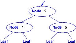 ** let val t = Node(1, Leaf, Leaf)
val u = Node(5, t, t)
in Node(3, t, u)
end, which represents both of
** let val t = Node(1, Leaf, Leaf)
val u = Node(5, t, t)
in Node(3, t, u)
end, which represents both of
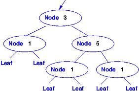
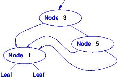 because the implementation shares substructure.
===================================================
because the implementation shares substructure.
===================================================
We use parameter patterns in functions that compute on inductive datatypes.
Say we
use IntTree to build ordered binary trees, e.g.,
Node(6, Node(3, Node(2, Leaf, Leaf), Leaf), Node(9, Node(8, Leaf, Leaf), Leaf))
Here is a tree-search algorithm for such trees,
expressed with patterns:
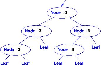
===================================================

(* member(i, t)  searches ordered IntTree t for int i and returns a boolean *)
fun member(i, Leaf) = false
|   member(i, Node(j, left, right)) = if i = j
                                      then true
                                      else  if i < j then member(i, left)
                                                     else member(i, right)
;

val member = fn : int * IntTree -> bool

===================================================
Here is an example execution:
member (2, Node(6, Node(2, Leaf, Leaf), Node(8, Leaf, Leaf)) )

   (arguments match second equation in definition of  member:)

= if 2 == 6
  then true
  else if 2 < 6  then member(2, Node(2, Leaf, Leaf))
                 else member(2, Node(8, Leaf, Leaf))

= if 2 < 6  then member(2, Node(2, Leaf, Leaf))
            else member(2, Node(8, Leaf, Leaf))

= member(2, Node(2, Leaf, Leaf))

   (arguments match second equation in definition of  member:)

= if 2 == 2
  then true
  else if 2 < 2  then member(2, Leaf)
                 else member(2, Leaf)

= true
Here is a function that collects the ints embedded in a tree:
===================================================

(* collect(t)  returns a list holding all the ints in  IntTree  t  *)
fun collect(Leaf) = []
|   collect(Node(i, left, right)) = collect(left) @ [i] @ collect(right)
;

val collect = fn : IntTree -> int list

===================================================
The subcalls,
collect(left) and collect(right), can be computed in parallel,
because there are no destructive assignments used while examining the tree.
Here is an execution:
collect Node(6, Node(2, Leaf, Leaf), Node(8, Leaf, Leaf))

=  (collect Node(2, Leaf, Leaf)) @ [6] @ (collect Node(8, Leaf, Leaf))

=  ((collect Leaf) @ [2] @ (collect Leaf)) @ [6] @ ((collect Leaf) @ [8] @ (collect Leaf))

=  ([] @ [2] @ []) @ [6] @ ([] @ [8] @ [])

= [2] @ [6] @ [8]  =  [2, 6, 8]
Indeed, function collect gives us the standard pattern for processing
queries on databases that are structured inductively like
trees. Here is an example:
===================================================

(* search : (int -> bool) * IntTree  ->  int list   does a "database search":
     search(query, databasetree)  applies the query function to each node of
     databasetree and assembles a list of all the ints in the tree that make
     the query true
*)
fun search(q, Leaf) = []
|   search(q, Node(n, left, right)) =
        search(q, left) @ (if q(n) then [n] else []) @ search(q, right)

===================================================
We might search for the even-valued ints inside this IntTree "database", seen in the previous diagram:
===================================================

val db = Node(6, Node(3, Node(2, Leaf, Leaf), Leaf),  Node(9, Node(8, Leaf, Leaf), Leaf))

fun isEven(n) = ((n mod 2) = 0)        (* mod  means "modulo" *)

val evenInts = search(isEven, db)      (* evenInts  is  [2, 6, 8] *)

===================================================
This little pattern is the basis for the Google search engine, which does a
parallel, functional-style search on its tree-based model of the web when evaluating
your query.
Finally,
here is a function that inserts an int into an ordered
tree.
Here is our example IntTree:
We wish to insert the value, 4, into it.
Remember: in functional programming, once a data structure is constructed in the
heap, it is never changed. So how do we "insert" the new value?
The answer is to construct a new tree that shares large pieces of the original,
like this:
Now, there are two trees in heap storage, and any threads of execution that are using
the orginal tree are unharmed by the insertion.
The new tree has its own "spine", shown in red above, that leads to the node with 4.
Here's the function that builds the new tree with the insertion:
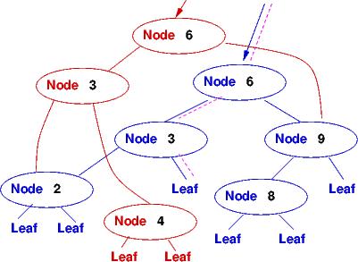
===================================================

(* insert(i, t)  inserts  i  into ordered tree  t
   pre: i  is an int;   t  is an IntTree whose nodes are ordered
   post: returns an ordered IntTree containing t's values and  i
*)
fun insert(i, Leaf) = Node(i, Leaf, Leaf)
|   insert(i, Node(j, left, right)) =
             if i < j then Node(j, insert(i, left), right)
                      else Node(j, left, insert(i, right))
;

val insert = fn : int * IntTree -> IntTree

===================================================
The new tree, with its own spine, shares the subtrees that are
irrevelant to the insertion.
The cost of constructing the new spine is of Order(log2N), where the tree holds N nodes.
User-defined datatypes define schemas for data-structure building,
much like classes do for object-oriented programming. Here are some
types for a library's database, modelled as a list of entries of books
and DVDs:
datatype Item =  Book of string * string   (* Book(title,author) *)
              |  Dvd of string             (* Dvd(title)         *)

datatype DBEntry = Entry of int * Item     (* Entry(idnumber, item) *)

type Database = DBEntry list
The point of this small example is that a multi-layered data structure can be defined
from multiple datatype equations.
Datatypes work great for defining tree-like structures that mix
strings, ints, subtrees, lists, etc.
If you review Chapter 1 on grammars, interpreters, and parsers,
you see inductively-defined data types everywhere.
For example, for this syntax of expressions:
EXPR ::= DIGIT | - EXPR | ( EXPR + EXPR )
A parser might generate operator trees of this datatype:
===================================================

datatype ETree = Digit of char  |  Negation of Etree  |  Addition of Etree * Etree

===================================================
The function that interprets ETrees is short and sweet:
===================================================

(* interpretETree computes the int meaning of its ETree argument  *)
fun interpretETree(Digit c)  =  (ord(c) - ord(#"0"))
|   interpretETree(Negation(t))  =   ~(interpretETree(t))
|   interpretETree(Addition(t1,t2))  =  interpretETree(t1) + interpretETree(t2)
;

val interpretETree = fn : ETree -> int

===================================================
Using ML-style datatypes, we can write a language's interpreter in about
as many lines as the the language's operator-tree constructions.
===================================================

(** For these syntax rules:
       PROGRAM ::=  COMM;*
       COMM ::=  ID = EXPR  |  print EXPR
       EXPR ::=  NUM |  ID  |  ~ EXPR  |  ( EXPR + EXPR )
  we define these datatypes:   **)

type Iden = string               (* identifers are strings *)

datatype ETree = Num of int  |  Var of Iden
              |  Negation of ETree  |  Addition of ETree * ETree

datatype CTree = Assign of Iden * ETree  |  Print of ETree

type Program = CTree list
;

(* Programs compute on storage vectors, defined as follows:  *)

type Store = (Iden * int) list   (* storage vectors, e.g., [("x",9), ("y",2)] *)

(* lookup : Iden * Store -> int     Does storage lookups.  *)
fun lookup (i, nil: Store) =  raise Empty (*error*)
|   lookup (i, (j,n)::rest) =  if i = j then n
                               else lookup(i, rest)
;
(* update : Iden * int * Store -> Store    Does storage updates.  *)
fun update(i, n, s: Store) =  (i,n)::s   (* Maybe you can write a better coding??? *)
;

(* INTERPRETATION FUNCTIONS FOR THE OPERATOR TREES *)

(* interpretEtree : ETree -> Store -> int
   interpretETree computes the int meaning of its ETree argument  *)
fun interpretETree(Num n) s  =  n
|   interpretETree(Var i) s = lookup(i, s)
|   interpretETree(Negation(t)) s =   ~(interpretETree t s)
|   interpretETree(Addition(t1,t2)) s =
      (interpretETree t1 s) + (interpretETree t2 s)  (* note two uses of s! *)
;
(* interpretCTree : CTree -> Store -> Store
   interpretCTree computes the updated store  *)
fun interpretCTree (Assign(i, e)) s =  update(i, (interpretETree e s), s)
                                       (* note two uses of s! *)
|   interpretCTree (Print e) s =  (print (Int.toString (interpretETree e s));
                                   s)  (* storage is unchanged *)
;
(* interpretCTreeList : CTree list -> Store -> Store
   sequences the execution of the CTrees  *)
fun interpretCTreeList [] s = s
|   interpretCTreeList (c::rest) s =
       interpretCTreeList rest (interpretCTree c s)
;
fun interpretProgram p = interpretCTreeList p []  (* start with empty storage *)

===================================================
We use the interpreter like this:
interpretProgram [Assign("x", Num 2),
                  Assign("y", Addition(Var "x", Num 1)),
                  Print(Addition(Var "x", Var "y"))]
Notice that
interpretCTree (Assign(i, e)) s = update(i, (interpretETree e s), s)"Input argument" s is used to compute the int that binds to i in the answer store.
interpretCTreeList (c::rest) s = interpretCTreeList rest (interpretCTree c s)This important property was not clearly presented in the Python interpreters in Chapters 1 and 2 because we used a global variable for the storage vector.
interpretETree(Addition(t1,t2)) s = (interpretETree t1 s) + (interpretETree t2 s)We might compute the arguments in parallel. This important property was not clearly presented in the Python interpreters in Chapters 1 and 2 because we used a global variable for the storage vector.
Other languages, like ML and Haskell, use a Pascal/Java-like type system, where each value has a specific type; all the elements of a list must have the same type; and only values of the same type can be compared for equality.
Let's look at ML, which uses a type checker.
Here is the syntax of types in ``core ML'':
===================================================

T ::=  string  |  T list

===================================================
For example,
"a"  has type  string

"a" :: nil  has type  string list

nil :: (("a" :: nil) :: :: nil)  has type  (string list) list
These requirements are formalized by logic-rule typing laws, defined
on the syntax of the language:
===================================================

A : string  (where A          E1 : T    E2 : T list
             is an Atom)     ------------------------
                                E1 :: E2 : T list

E : T list             E : T list
-----------          ---------------
hd E : T             tl E : T list


E1 : T list   E2 : T'   E3 : T'
---------------------------------
 ifnil E1 then E2 else E3 : T'

===================================================
For example, since (1::2::nil) is typed int list, then the third law, for hd,
asserts that hd (1::2::nil) is typed int.
These laws are coded into the ML type checker, which is actually a simplistic theorem prover that uses laws to prove that an expression has a specific data type. The data type is a "prediction" about the "shape" of the answer that will be calculated.
Next, the ML interpreter calculates the meaning of the expression,
which always matches the prediction made by the type checker.
So, if you start the ML interpreter and type,
- nil :: (("a" :: nil) :: nil);
the response is
val it = [[], ["a"]] : (string list) list
The type checker first proved that the expression has type
(string list) list, and then the interpreter calculated the normal form,
which indeed was a string list list. The type checker never makes
a false prediction because the logic-rule typing laws are sound
(faithful) to the calculation laws of ML.
One question remains: What is the type of nil?
The answer is, T' list, for any type T' whatsoever.
So, nil has ``many types,'' depending on where it is inserted
in an expression. (See the earlier examples.)
For this reason, its ``typing rule'' goes:
===================================================

nil : T List

===================================================
where you can fill in T as you wish.
ML would print val it = [] : 'a list, using 'a as the dummy type name.
NOTE: More precisely, ML's type checker proved that nil has the type, Forall 'a ('a list), where Forall 'a is the universal quantifier from predicate logic --- the ML type checker is a theorem prover for positive propositional logic with shallow universal quantification.
The ML type checker deduces the type of an expression by annotating
all the expression's phrases with types.
Here is a small example to show how the types can be attached to the nodes
of an expression's operator tree, hd ("a"::nil):
The typing attached to each node of the tree is justified by one of the previous
typing laws.
α is a logical variable ("Skolem variable") that stands for an unknown
type. The logical variable is later "narrowed" or unified to a more specific typing, here, to string.
Here is the typing of the more complex example, nil :: (("a" :: nil) :: nil), which requires multiple logical variables:
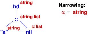
In the example, the first nil has typing, α list, but
later, when the rest of the expression, ("a" :: nil) :: nil, is
typed as (string list) list, this narrows α to equal
string.
The second nil has typing, β list, but β must be narrowed
to string so that "a" :: nil can be typed (as string list).
The third nil is initially typed γ list, but since
"a" :: nil is typed string list, then γ must be narrowed
to string list. The typing of the entire expression becomes
(string list) list.
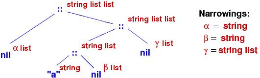
When you define an ML function, the type checker checks the
function's code and calculates the type. The interpreter constructs
the function's closure and shows the type, e.g.,
- fun double(n) = n * 2;

val double = fn : int -> int
The function's type is int -> int, that is,
an int argument is required to produce an int answer.
Sometimes an function can be used with arguments of different types,
e.g.,
- fun second(xs) = hd(tl xs);

val second = fn : 'a list -> 'a
You should read second's typing as
Forall α (α list -> α).
The function can be called as second [1,2,3] or as second["a","b","c"]
or as
second( nil :: (("a" :: nil) :: nil)).
This is because the Forall 'a quantifier can be instantiated in multiple
ways.
A function that can be used with multiple typings of arguments is called
polymorphic.
Here is the typing calculation of the function,
fun f(m, n) = n :: (m n):
The function's type is printed as (('b -> 'b list) * 'b) -> 'b list by ML.
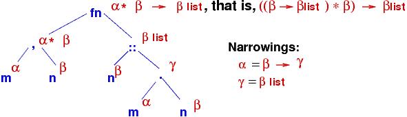
The parameters, m and n, might have any typings at all, so logical variables, α and β, are used. In the body of the function, the uses of m and n will narrow the values of the two logical variables. Indeed, the expression, (m n), narrows α to the function typing, β -> γ, where γ is a new logical variable --- the answer typing is not yet known.
Since the answer of (m n) is used with a :: operation, this narrows γ to the list typing, β list, and the final typing, (α * β) -> (β list), is narrowed to the typing, ((β -> β list) * β) -> β list.
The algorithm that traverses an expression, attaches typings to the subphrases, and applies narrowings was invented by Robin Milner and is called Algorithm W. The algorithm was independently discovered by Roger Hindley and for this reason it is sometimes called the "Hindley-Milner algorithm."
Here again are the typing rules used by ML for ints, strings, and lists.
The rules are written as logical axioms and inference rules,
and each law/rule has a name:
===================================================

(intrule)  N: int,   where N is a numeral

(stringrule)  S : string   where S is a double-quoted sequence

           E1: int   E2: int
(addrule) ------------------   (there are similar rules for -, *, ..., and string operations)
            (E1 + E2): int


(nilrule)  nil: T List (for any type,                E1: T    E2: T list
                       T,  at all)      (consrule) ---------------------
                                                     E1 :: E2: T list

           E: T list                    E: T list
(hdrule) -----------         (tlrule) ---------------
           hd E: T                    tl E: T list


          E1: T list   E2: T'   E3: T'
(ifrule) ----------------------------------
         ifnil E1 then E2 else E3 : T'


===================================================
This is "ML logic".
Here is the logical proof, written in ML logic, that we extract from the Algorithm-W-checked operator tree for
hd("a"::nil):
===================================================

1. "a" : string              stringrule
2. nil : string list         nilrule
3. "a"::nil : string list    consrule 1,2
4. hd("a"::nil) : string     hdrule 3

===================================================
Each line number matches a node in the type-checked operator tree.
The logical variable is replaced by its
narrowing, and the result looks like a well planned proof.
Here is the second example,
nil :: (("a" :: nil) :: nil):
===================================================

1.  nil :  string list                             nilrule
2.  "a" :  string                                  stringrule
3.  "a"::nil :  string list                        consrule 2,1
4.  nil :  string list list                        nilrule
5.  ("a":: nil):: nil :  string list list          consrule 3,4
6.  nil :  string list                             nilrule
7.  nil:: (("a"::nil):: nil) :  string list list   consrule 6,5

===================================================
Every type-annotated operator tree can be reformatted as a logical
proof of data typing. It is a mechanical process, working from
the tree's leaves to the root.
Here are two more proofs in ML logic, written from scratch:
===================================================

|-  (2 + 1) :: nil :  int list

1.  2 :  int                    intrule
2.  1 :  int                    intrule
3.  2 + 1 :  int                addrule 1,2
4.  nil :  int list             nilrule
5.  (2 + 1):: nil :  int list   consrule 3,4

===================================================
The above proves that the answer computed from (2 + 1) :: nil,
whatever it will be, will be an int list.
Now, here is a proof based on two premises:
===================================================

m : int -> int list,  n : int  |-   n:: (m n) :  int list

1. m : int -> int list       premise
2. n : int                   premise
3. (m n) : int list          callrule 1,2  (see below for this rule)
4. n :: (m n) :  int list    consrule 2,3

===================================================
We proved, if nonlocal values m and n are typed as stated,
then n::(m n) will compute to an int list.
===================================================

1.  2    means (intrule)
2.  1    means (intrule)
3.  +    means (addrule)
4.  nil  means (nilrule)
5.  ::   means (consrule)

===================================================
That is, (2 + 1):: nil encodes the proof steps that prove the proposition, int list! Here it is, properly formatted:
===================================================

1.  2 :  int                    intrule
2.  1 :  int                    intrule
3.  2 + 1 :  int                addrule 1,2
4.  nil :  int list             nilrule
5.  (2 + 1):: nil :  int list   consrule 3,4

===================================================
===================================================

        P   Q                 P ∧ Q             P ∧ Q
(∧i) -----------      (∧e1) -------     (∧e2) --------
       P ∧ Q                    P                 Q


        ...  P assume
        ...  Q                   P —> Q    P
(—>i) ------------       (—>e) --------------
        P —> Q                         Q

===================================================
Here is a sample proof that you did as a beginner:
A ∧ B, B —> C  |-   A ∧ C

1.  A ∧ B      premise   (a premise is a "starting fact")
2.  B —> C      premise
3.  B           ∧e2  1
4.  C           —>e 2,3
5.  A           ∧e1 1
6.  A ∧ C      ∧i 5,4
Here's one that uses a local assumption to construct an implication:
(A ∧ B) —> C,  B  |-  A —> C

1. (A ∧ B) —> C     premise
2. B                premise
+--------------------------------
|... 3.  A              assumption   (an assumption is a "what if/let's pretend" fact)
|... 4.  A ∧ B          ∧i 3,2
|... 5.  C              —>e 1,4
+-------------------------------
6. A —> C       —>i 3-5
Each proof constructed an ML program:
p : (A * B), f : B -> C |- (fst p, f(snd p)) : A * CThat is, using "global values" p and f, we build the expression, (fst p, f(snd p)), which is typed A * C.
(Note: in Standard ML, fst is coded #1, and snd is coded #2. Oh well!)
f : (A * B) -> C, x : B |- (fn (y:A) => f(y,x)) : B -> C
===================================================

premise1: A ∧ B,  premise2: B —> C  |-   A ∧ C

Proof expression/tree:
  ∧i(∧e1(premise1), —>e(premise2, ∧e2(premise1)))

The line-by-line proof:
1.  A ∧ B      premise
2.  B —> C      premise
3.  B          ∧e2  1
4.  C          —>e 2,3
5.  A          ∧e1 1
6.  A ∧ C       ∧i 5,4

===================================================
Match the structure of the expression to the proof lines underneath it --- it's the same, just more compact, because there are no line numbers, only the names, premise1 and premise2. Here's the second proof:
===================================================

premise1: (A ∧ B) —> C,  premise2: B  |-  A —> C

Proof expression/tree:
  —>i(assumpt1:A,  —>e(premise1, ∧i(assumpt1, premise2)))

Line-by-line proof:
1. (A ∧ B) —> C     premise
2. B                 premise
+--------------------------------
|... 3.  A              assumption
|... 4.  A ∧ B          ∧i 3,2
|... 5.  C              —>e 1,4
+-------------------------------
6. A —> C        —>i 3-5

===================================================
Each proof constructed a proof term from its premises and the rules. Now, each proof term is just a computer program:
===================================================

∧i(P1, P2)      means  (P1, P2)  --- pairing

∧e1 P           means  fst P     --- indexing
∧e2 P           means  snd P     --- indexing

—>e(P1, P2)     means  P1(P2)    --- function call

—>i(x, P2)      means  fn x => P2
                   or   lambda(x) P2  --- function abstraction

===================================================
Here are the previous two proof terms, rewritten as programs:
===================================================

Proof term:
 premise1: A ∧ B,  premise2: B —> C  |-
   ∧i(∧e1(premise1), —>e(premise2, ∧e2(x))) :  A ∧ C

Program:
 p : A * B,  f : B -> C  |-  (fst p, f(snd p)) : A * C

===================================================
===================================================

Proof term:
 premise1: (A ∧ B) —> C,  premise2: B  |-
   —>i(assumpt1:A,  —>e(premise1, ∧i(assumpt1, premise2))) :  A —> C

Program:
 f : (A * B) -> C,  x : B  |-  (lambda(a: A) f(a, x)) : B -> C

===================================================
Here are the propositional-logic rules again,
written so that they look like ML's typing
rules, but again, they are just the same logic rules:
===================================================

        E1: P  E2: Q               E: P ∧ Q            E: P ∧ Q
(∧i) -------------        (∧e1) ----------     (∧e2) -----------
       (E1, E2): P ∧ Q             fst E: P             snd E: Q


        ... x: P assume
        ... E: Q                       F: P —> Q   E: P
(—>i) -------------------       (—>e) -----------------
      fn (x:P) => E : P —> Q             F(E):  Q

===================================================
The logic laws for conjunction build and disassemble pairs, and the
logic laws for implication build and call lambda abstractions
(functions).
The program terms are redundant, but most humans like to see them alongside
the propositions.
Here is the proof just seen, reformatted with the new rules:
(A ∧ B) —> C,  B  |-  A —> C

1. f :  (A ∧ B) —> C         premise
2. x :  B                    premise
+--------------------------------
|... 3.  y : A                 assumption
|... 4.  (y,x) : A ∧ B         ∧i 3,2
|... 5.  f(y,x) : C            —>e 1,5
+-------------------------------
6. (fn (y:A) => f(y,x)) :  B —> C    —>i 3-5
The proof uses premises (nonlocal values), f and x,
to construct a function that builds a C-typed answer when called.
Here is the moral of this story:
We can add the usual logical rules for disjunction (∨), and they will give us a version of ML's datatype builder and ML's case expression. We can also add a weakened form of negation (called intuitionistic negation), and this defines ML-style exceptions. (Classical negation and its proof-by-contradiction law will not generate computer code!) The result is intuitionistic propositional logic.
If we are brave, we can progress to predicate logic: add the laws for the universal
quantifier, ∀, and the existential quantifier, ∃, and
use them to build programs/proofs that realize/prove
specifications written in predicate logic. Here are three
example specifications:
square :  ∀x: int ∃y: int (y = x * x)

largest : ∀ns: int list ∃k: int
              (k in ns  ∧  (∀m: int (m in ns —> k >= m)))

removeElement :  ∀(k, ms): (int ∧ int list) ∃ns: int list
                     (((k in ms) ∧ isPermutation(k::ns, ms))
                      ∨  ((¬(k in ms)) ∧ ns = ms))

sortList :  ∀α ∀xs: α list ∃ys: α list
                (isOrdered(α, ys) ∧ isPermutation(xs, ys))
When we prove these specifications, we have proved-correct program code
as a result --- no need for testing!
Here is a small example to show how this is done. First, to prove
properties about ints, we must add rules/laws for ints,
such as these two:
===================================================

                                           E1 = E2
(reflexive law)  E = E      (greaterrule) -------------
                                           E1 + 1 > E2

===================================================
(Of course, there are more rules about numbers --- Peano's laws of arithmetic.)
We also use these logic rules for ∀i and
∃i:
===================================================

                               ... m: A   assume (m  must be a new unused name)
      BE    E: A               ... B
(∃i) --------------     (∀i) ---------------
        ∃(x:A) Bx               ∀(m:A) B


===================================================
We use these rules to prove this logic claim:
|-  ∀(x: int) ∃(y: int) (y > x)

+----------------------
|... 1. x : int           assumption
|... 2. x = x             reflexive law
|... 3. x + 1 : int       addrule 1
|... 4. (x+1) > x         greaterrule 2
|... 5. ∃(y:int) y > x    ∃i 3,4
+----------------------
6. ∀(x:int) ∃(y:int) (y > x)  ∀i 1-5
The ML code inside this proof is the
function, (fn(x:int) => x + 1), along with its correctness proof.
Here is the proof with the code and proof terms explicitly listed:
===================================================

|-  ∀(x: int) ∃(y: int) (y > x)

+----------------------
|... 1. x : int                                       assumption
|... 2. reflex(x) :  x = x                            reflexive law
|... 3. x + 1 : int                                   addrule 1
|... 4. greater(reflex(x)) : (x+1) > x                greaterrulle 2
|... 5. [x+1, greater(reflex(x))] : ∃(y:int) y > x    ∃i 3,4
+----------------------
6. Fn(x:int) => [x+1, greater(reflex(x))]: ∀(x:int) ∃(y:int) (y > x)  ∀i 1-5

===================================================
Look closer at the proof term:
     Fn (x: int) =>  [ x+1,  greater(reflex(x):(x=x)):(x+1>x) ]
            ^           ^     ^
            |           |     | proof that answer,  x+1,  is  >  argument  x
            |           |
            |           | answer ("witness") computed by function
            |
            | argument to function
This mix of code and proof is called proof carrying code
and has been used in applet-based, distributed systems where processes share
code but security and correctness must be maintained.
It is based on a beautiful logic known as Martin-Loef Intuitionistic Type Theory.
Here is a second example, which specifies a program that returns a nonnegative
int smaller than its argument, provided the precondition that the argument is a
positive int:
===================================================

|- ∀(x: int) (x > 0) —> (∃(y: int) (x > y  ∧  y >= 0))

+----------------------
|... 1. x: int          assumption
|...+--------------------
|...|... 2. x > 0          assumption
|...|... 3. x - 1 : int    intrules 1
|...|... 4. x > x - 1      PeanosLaws 1,3
|...|... 5. x - 1 >= 0     PeanosLaws 1,2,3
|...|... 6. (x > x - 1) ∧ (x - 1 >= 0)   ∧i 4,5
|...|... 7. ∃(y:int) (x > y) ∧ (y >= 0)  ∃i 3,6
|...+--------------------
|...8. (x > 0) -> (∃(y:int) (x > y) ∧ (y >= 0))  —>i 2-7
+------------------------
9. ∀(x: int) (x > 0) —> (∃(y: int) (x > y  ∧  y >= 0))  ∀i 1-8

===================================================
We skipped some arithmetic reasoning by appealing to PeanosLaws
for numbers.
Here is the proof term, a function that requests an int, x, and a proof, p,
that x is positive:
Fn (x: int) =>  fn (p: x > 0) => [x - 1, ∧i(Peanos(x, x-1):(x > x-1), Peanos(x, p, x-1):(x-1 >= 0))]
 ^               ^                  ^      ^   ^                         ^
 |               |                  |      |   |                         | proof that x-1 >= 0
 |               |                  |      |   | proof that x > x - 1
 |               |                  |      | pairing of the two subproofs
 |               |                  |
 |               |                  | witness ("answer")
 |               | param that binds to proof code that  x > 0
 | param that binds to int  x
Notice how proof, p, is used to prove that answer x-1 is >= 0.
In the proof-carrying-code world, proofs are data values like ints.
A logical framework is a proof-building tool that uses proof rules like the ones seen here to construct proved-correct programs. The aerospace industry uses logical frameworks, and even Microsoft has integrated them in the development of some software systems. (It is possible to do these activities in assignment languages, using Floyd-Hoare logic, but the presentation given here is more compact. Microsoft uses a logical framework, CodeContracts, for C# using Floyd-Hoare logic, theorem proving, and a theory of computational approximation known as abstract interpretation.)
The field of intuitionistic logic ("constructive logic") is the study of algorithm extraction from logical proofs and computation ("normalization") of the algorithms. A great historical reference is Troelstra and van Dalen's two-volume set, Constructivism in Mathematics, but you would do well to start with Dirk van Dalen's intro text, Logic and Structure.
Finally, consider again ML's Algorithm W: it examines an ML program
and treats it as an incomplete proof of a formula in this logic:
F : TypeFormula
P : Proposition      I : TypeVariable

F ::=  ∀(I) F  |  P
P ::=  P * P  |  P -> P  |  int  |  string  |  P list  |  I
I ::=  α  |  β  | ...
This is a positive (no-negation) propositional logic with shallow (leftmost)
universal quantification over propositions --- much simpler than first-order predicate logic!
Algorithm W uses logical variables and narrowing to determine the
formula, if any, that is proved. It is the best-known example
of an "automatic logical framework" but for a severely restricted predicate logic.
fn(x:int) => [x+1, succ(refl(x))]: ∀(x:int) ∃(y:int) (y > x)It can be called with an argument, e.g., 3:
(fn(x:int) => [x+1, succ(refl(x))])(3)
     =  [3+1, succ(refl(3))]
     =  [4, succ(refl(3))]  :  ∃(y:int) (y > 3)
The = steps are computation steps (called "proof normalization" by logicians) and
computes the answer, 4, and a proof that the answer is correct, that is,
4 > 3 (because 3=3 and 3+1>3).
The function-call step is exactly the ∀e-rule of logic:
===================================================

      F : ∀(x:A) Bx    E : A
(∀e) ----------------------------
              F E :  BE

===================================================
Now that we understand that proofs in logic are really programs, we see that program development is proof construction --- starting from premises (laws about the program domain), we apply logic rules to prove a goal (program specification).
A theorem-proving program builds proofs of goals from premises. An interpreter "executes" (simplifies/normalizes) the proofs. Humans don't have to do these things!
If a human can state the premises of the program domain in logic and if a human can state the goal of a program in logic, then a computer can write the program and execute it. This approach is called logic programming, and there are languages, like Prolog, Datalog, and Parlog, that use this approach: the human writes the logical specifications and the computer does the coding and the execution!
Kurt Goedel's famous First Incompleteness Theorem (1931) proved that it is impossible to build an automatic logical framework (theorem prover) that generates algorithms (proofs) for all true formulas in first-order predicate logic enriched with Peano's laws of arithmetic. So, we can never completely automate program construction from specifications. (The Prolog-like languages work with subsets of predicate logic, and even in the subsets, some programs are not synthesized --- they "loop".)
Here is how we write correct programs that use lists. We employ the list induction rule. The rule proves logical properties about lists.
First, here are
examples of logical properties for lists:
===================================================

(* m is a sorted list: *)
Sorted(m) ==  (i)  m = [a0, a1, ..., an]   and
              (ii) a_i <= a_i+1, for all 0 <= i < n

(* list  ys  is list  xs  but in reverse order: *)
Reversed(xs, ys) ==  (i) xs = [a0, a1, ..., an]   and
                     (ii) ys = [an, ..., a1, a0]

(* int  m  is the largest in int list  ns:  *)
Largest(ns, m) == (i)  m in xs  and
                  (ii) m <= every  n in ns

===================================================
These are correctness properties --- for example, we might write some
safety-critical code, function reverse, that reverses a list.
We want this correctness property of it:
Reversed(arg, (reverse arg)), for every possible list argument, arg.
The correctness property is a data type of the function.
The "correctness type" of reverse is
Forall arg : 'a list Exists ans : 'a list, such that Reversed(arg, ans)
We can prove such properties with the
list-induction proof rule. Here is one version; an explanation is
just underneath the rule!
===================================================

                            +-------------------------------------
                            |  (x::xs) : 'a list        assumption
            b : P(nil, b)   |  (f xs) : P(xs, (f xs))   assumption
                            |    ...
                            |  e(x, xs, (f xs)) : P(x::xs, e(f xs))
                            +-------------------------------------
(list ind)--------------------------------------------------------
          fun f  nil    =  b
          |   f (x::xs) =  e(f xs)
                           : Forall arg, Exists ans, such that P(arg, ans)

===================================================
A function that computes on a list should be written in two equations,
like this:
fun f nil = b
|   f (x::xs) = e(x, xs,(f xs))
There is the "nil case", which returns some simple answer, b,
and the "cons case", which builds an answer, e(...), from x, xs,
and the recursive call, (f xs).
To prove that function f has correctness property, P,
we have two proofs to make: (Match these to the inference rule just above.)
The data type of the function is more precisely written as Forall arg Exists ans, P(arg, ans).
Here is a worked example.
Recall this property about lists:
Reversed(xs, ys) ==  (i) xs = [a0, a1, ..., an]   and
                     (ii) ys = [an, ..., a1, a0]
We can prove
that the rev function below has the Reversed correctness type:
===================================================

fun rev nil = nil
|   rev (x::xs) = (rev xs) @ [x]
                        : Forall arg Exists ans, Reversed(arg, ans)

===================================================
Here is the proof:
===================================================

1.  nil : Reversed(nil, nil)    because (i) nil = [] and (ii) nil = [],
                                so all zero of its elements are reversed

+---------------------------------------------------------------------------
|  2.  (x::xs) : 'a list                   assumption

|  3.  (rev xs) : Reversed(xs, (rev xs))   assumption (induction hyposthesis)

|  4.  (rev xs) @ [x] : Reversed((x::xs), (rev xs) @ [x])

                           because Line 3 tells us
                             (i)  xs = [a0, a1, ..., ak],
                             (ii) rev xs = [ak, ..., a1, a0]
                           so:
                             (i)  x::xs = [x, a0, a1, ..., ak]
|                            (ii) (rev xs) @ [x] = [ak, ..., a1, a0, x]
+---------------------------------------------------------------------------
5. fun rev ... : Forall arg Exists ans,  Reversed(arg, ans)    list ind 1, 2-4

===================================================
The "because" explanations are really small proofs in arithmetic/algebra.
The proof is a type-checking analysis, where the data type is the correctness property. It matches how we think about the code when we write it.
It is easy to use parameter patterns to write exactly these structures
for an inductively defined data type. Here are three sample instances
of these control structures
for binary trees of values:
===================================================

datatype 'a Tree = Leaf  |  Node of 'a * Tree * Tree

fun map(f, Leaf) =  Leaf
  | map(f, Node(a, t1, t2)) = Node(f(a), map(f, t1), map(f, t2))

fun filter(b, Leaf) = []
  | filter(b, Node(a, t1, t2)) = (if b(a) then [a] else [])
                                 @ filter(f, t1) @ filter(f, t2)

fun reduce(r, startvalue, Leaf) = startvalue
  | reduce(r, startvalue, Node(a, t1, t2)) =
              let v1 = reduce(r, startvalue, t1) in
              let v2 = reduce(r, v1, t2) in
              r(a, v2)
              end end

===================================================
Notice that f, b, and r are functions that are arguments
to the control structures.
ML has built-in versions of map and reduce (two variants: foldl and foldr) for linear lists.
The computation-as-algebra concept fails with imperative languages,
because assignment destroys values.
For example:
int x = 0;
if (...) { x = x + 1 }
print x;
there is no way we can substitute 0 for the occurrences of x
in this program.
Instead, we must execute the program with an instruction
counter and primary storage.
Imperative languages work best with table-based storage structures with little or no need for roll back, for example, a voting table or a graphics system that maintains the matrix of pixels on a display.
When you are programming with assignments, think of an assignment as a slightly dangerous device, like a blow-torch whose flame "burns away" values in storage. Use the device with care. You can often streamline your code with these techniques:
For heaven's sake, not all problems should be solved with functional-programming techniques! A device driver or graphics kernel should be coded in C, and a table-based, component system should be built in an imperative object language. (By the way, don't program tables in a functional language.) Be aware that no single paradigm works for everything, so you should be competent in multiple programming paradigms so that you can program the best solution for the task at hand.