At (a):The array is allocated as a stand-alone object, and y in namespace α is bound to handle β, where the array's cells live.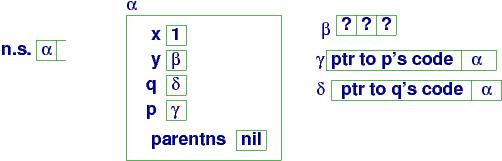
Programs are usually assembled from pieces, or components, like functions, modules, and classes, and a programming language must provide structure for defining and assembling components.
In this chapter, we see that component mechanisms in programming languages are a product of several principles first proposed by Robert Tennent of Queen's University, Canada, in the 1970s. Tennent studied the origin of naming devices for functions, procedures, modules, and classes and discovered that they were based on one and the same theme. He later saw a similar theme in the development of varieties of block structure. Schmidt (your instructor at KSU) noted that Tennent's ideas also applied to the forms of parameters that can be used with functions.
The results were the abstraction, parameterization, and qualification principles of language extension. The three principles help us understand the structure, origins, and semantics of component forms and they provide us with advice as to how to add such forms to languages we design.
In this chapter, we briefly survey the principles and in subsequent chapters we apply them to develop sophisticated languages.
If our language has a syntax domain of expressions, then we can name expressions (they are (pure) functions) and we can call them by stating their names in any position where an expression might be used.
Tennent titled the named phrases abstracts. That is, procedures are ``command abstracts'' and functions are ``expression abstracts'' and so on.
Indeed, every syntax domain of the language might be nameable and callable. This is the impact of the abstraction principle, which is the elegant alternative to ``copy-and-paste'' programming.
Say we have this baby assignment
language:
===================================================

P : Program             D : Declaration
E : Expression          I : Identifier
C : Command             N : Numeral

P ::=  D ; C

D ::=  int I  |  D1 ; D2

C ::=  I = E  |  C1 ; C2  |  while E { C }  |  print E

E ::=  N  |  E1 + E2  |  E1 != E2  |  I

N ::=  0 | 1 | 2 | ...

I ::=  alphanumeric strings

===================================================
We have Declarations of variables, that is,
assignable (``mutable'') ints. Soon we will have declarations of
procedures, pure functions, etc.
===================================================

D ::=  int I  |  D1 ; D2  |  proc I = C end

C ::=  I = E  |  C1 ; C2  |  while E { C }  |  print E  |  I()

===================================================
The declaration, proc I = C, makes I
name command C. (Other possible forms of syntax are
proc I(){C} or def I(): C or
void I(){C}, but the point is that I names C.)
To reference (``call'') a procedure, we state its name where a command
can appear; this is why we added
C ::= . . . | I()
to the syntax for commands. (Perhaps you prefer call I or just
I for the syntax --- take your pick.)
Here is an example that uses a procedure:
===================================================

int i;  int ans;  int n;
proc factorial =
    i = 0;  ans = 1;
    while i != n {
        i = i + 1;
        ans = ans * i
    }
    end;
n = 4;
factorial();
print ans

===================================================
So, that's the syntax; what about the semantics?
The semantics of procedure definition is to save the procedure's name and
its code body in the virtual machine's namespace.
The semantics of a procedure call executes the code body with the current
value of storage at the position
where the procedure is
called. The previous example executes like this:
n = 4
factorial() +--> # factorial's body commences:
                 i = 0
                 ans = 1
                 while i != n {
                    i = i + 1
                    ans = ans * i }
  < -----------+
print ans
The program executes as if the procedure's body is copied in place
of its call --- this is the ``copy rule'' semantics
of procedure call. (A newcomer
would say it is copy-and-paste!) A computer implements
copy-rule-style semantics with an instruction counter and a
stack of namespaces (activation
records), as we see later in this Chapter.
The factorial example has a well-known coding that uses recursive call:
int i;  int ans;  int n;
proc factorial =
      if i != n {
          i = i + 1;
          ans = ans * i;
          factorial()
      }
      end;
factorial()
The copy-rule semantics of execution shows that each self-call is just a
call to a "fresh copy" or "clone" of the procedure's body:
===================================================

n = 3;
i = 1;
ans = 1;
factorial() ---> # In storage,  n == 3,  i == 1  and  ans == 1
                 if i != n   # computes to True
                 i = i + 1 ;
                 ans = ans * i ;
                 factorial() ---> # Now,  i == 2,  ans == 2
                                  if i != n  # computes to True
                                  i = i + 1 ;
                                  ans = ans * i ;
                                  factorial() ----> # Now, i == 3, ans == 6
                                                    if i != n  # False!
                                                    # do nothing
                                  <-----------------+
               <------------------+
<--------------+
# In storage,  n == 3,  i == 3,  and  ans == 6

===================================================
A computer implements
copy-rule-style semantics with an instruction counter and
stack of namespaces (activation
records), as we see later in this Chapter.
Given that a procedure is declared like a variable is declared,
can we
update ("mutate") procedure code by assignment? In scripting languages,
you can. Here's a Python example:
===================================================

x = 2
def p(): print x

q = p             # q is assigned p's code
p = "x = x + 1"   # p is reset to a _string_ holding code ("quoted code")
exec p            # execute the quoted code
q()               # can call q directly; prints  3

===================================================
In the example, p and q are variables
and the value assigned to q is a handle
to a closure object that holds code. Closures come later in the chapter.
Most compiler-based languages
disallow assignment to procedure names, because it ruins the compiler's
usual optimization of replacing a procedure call by an instruction-counter jump.
But there is this trick you can do in C# with delegates:
delegate void Proc()          // defines a "procedure type"  Proc
Proc q;                       // declares var  q,  it can be assigned Proc code

q = delegate(){ i = i + 1; }  // assign a  Proc _value_ to  q
q()                           // call it
In these examples, command code are values, just like ints are values.
C# implements delegate values with closures, which come later in the chapter.
===================================================

E ::=  N  |  E1 + E2  |  E1 != E2  |  I  |  I()

D ::=  int I = E  |  D1 ; D2  |  proc I() { C }  |  fun I() E

===================================================
Function-declaration semantics is different than assignment semantics, for sure:
int i = 0;
int f = i + 1;
fun g() i + 1;
i = 8;
print f;         # prints  1
print g();       # computes meaning of code,  i + 1, and prints 9
We might say that the expression for f is computed eagerly (immediately) and the expresson for g is computed lazily (when demanded). These two notions are relevant to the semantics of parameter passing, which comes later in the chapter.
Most general-purpose languages omit pure functions
in favor of procedures that quit with a return E command.
Here is factorial, written as a procedure that returns an answer:
===================================================

int count = 0;
proc fac(n) { count = count + 1;
              if n == 0 { return 1; }
              else      { int a = fac(n-1);
                          return n * a; }
            }
print fac(5);

===================================================
Many people call fac a ``function,'' but more
precisely it is a procedure that returns an answer.
The function-procedure's
commands can change global variables (like count in the example).
A function-procedure that changes global variables is called an
impure function.
Now, impure functions need not be a "hack". Indeed, in C (and Python),
they are a consequence of the abstraction principle, because the
the syntax of C states that every command returns a value, just like
an expression does! You've probably used this C trick:
int x = 2;
int y = (x = x + 1);   // updates x to 3 and sets y to 3 also,
                       // because the assignment is used as an expression
The syntax of commands and expression in C are in fact merged together:
===================================================

E : Expression/Command

E ::=  L = E  |  E1 ; E2  |  if ( E ) E1 else E2  | ...
    |  N  |  L  |  ( E1 + E2 )  |  return E  | ...

===================================================
Procedures (functions) in C are just "impure" functions.
By the way, what is the difference in semantics in these two C-examples?
int x = 2;                      int x = 2;
int y = ++x;                    int y = x++;
We can go further than procedures and functions --- looking at the syntax definition at the top of this chapter, we might define Declaration abstracts and Numeral abstracts and even Identifier abstracts!
Declaration abstracts are important --- they are known as modules or packages. All modern languages let you collect a family of declarations into a module/package and later import the module (link it) to the main program.
For example, if we extend the baby language at the start of the chapter with declaration abstracts, we have this syntax:
===================================================

D ::=  int I  |  D1 ; D2  |  proc I = C end
    |  module I = D  |  import I

===================================================
This means we can "package" some declarations, name them, and activate them:
module Clock =  int time;
                proc init =  time = 0  end;
                proc tick =  time = time + 1  end;

int x;
import Clock;   // activates the declarations in Clock
init();
tick();  tick()
and so on.
Modern languages let you save a module/package in a separate file.
To reduce confusion, these languages request that you use dot-notation
to refer to the declarations in an imported module, like this:
// one file:
module Clock =  int time;
                proc init =  time = 0  end;
                proc tick =  time = time + 1  end;

// another file:
int x;
import Clock;   // activates the declarations in Clock
Clock.init();
Clock.tick();  Clock.tick()
It is possible to avoid the dot-notation in these languages with a
special invocation construction:
int x;
from Clock import *;   // or maybe,  import Clock.*;
init();  tick();  tick()
The semantics of module/package importation is again a copy rule --- the declarations are activated/"copied" into the program.
But there is one special restriction in most modern languages: you can
activate a module in any program at most once. This is a hack-fix to this modern problem:
===================================================

// file  Clock:
module Clock =  int time;
                proc init =  time = 0  end;
                proc tick =  time = time + 1  end;

// another file, Part 1:
module Part1 =  int x;
                import Clock;
                init();

// another file, Part 2:
import Clock;
import Part1;   // is there one Clock or two?  Just one!
x = 3;
tick()          //  ticks the one and only Clock

===================================================
We will study modules/packages in more detail in a later chapter.
Numeral abstracts are sometimes called final variables or consts. Does your favorite language have these?
Identifier abstracts are called aliases. An alias copies the address of one variable as the address of another. This idea reappears when we study "var" or "ref" (call-by-reference) parameters.
There is another kind of "pasting": a program might have a "hole" in it where some data must be inserted later, when the program executes. The "hole" is usually represented by an identifier, called a parameter. An argument must be supplied to "paste" (bind) into the "hole" marked by the parameter. Here is the principle of parameterization:
We return to the little assignment language and revise
procedures so that they have parameters.
The parameterization principle sugguests that
any expression phrase can be an argument for
a procedure's parameter. For the example language, we have
===================================================

E ::=  N  |  E1 + E2  |  E1 != E2  |  I

C ::=  I = E  |  C1 ; C2  |  while E { C }  |  print I  |  I ( E )

D ::=  int I  |  D1 ; D2  |  proc I1 ( I2 ) { C }

===================================================
The procedure is proc I1(I2){ C }, where I2 is a parameter name, and the
procedure
must be called with I1(E), where E is an expression that is bound
to I2.
The syntax is usually generalized so that
you can have zero
or multiple parameters:
C ::=  I = E  |  C1 ; C2  |  while E { C }  |  print I  |  I ( E,* )
       where  E,*  means zero or more of Es, separated by commas

D ::=  int I  |  D1 ; D2  |  proc I1 ( I,* ) { C }
       where  I,*  means zero or more of Is, separated by commas
Within the procedure, the parameter is used by mentioning its name.
Here is a factorial procedure with a parameter:
===================================================

int ans;
proc fact(n) {
    ans = 1
    while n != 0 {
        ans = ans * n;  n = n - 1
    }};
int x = 2;
fact(x + x);
print ans

===================================================
When fact is called, x + x is bound
to parameter name, n. How is this done? Here are some possibilities:
Almost all modern languages use ``assignment binding,'' also known as
call by value --- a new variable, n, is declared, and the value
of the argument, x + x, is assigned to it.
The program executes like this:
int x = 2
fact(x + x)
     x + x computes to 4 +-->  int n = 4  # note the "declaration" of n
                               ans = 1
                               while n != 0 {
                                  ans = ans * n
                                  n = n - 1
                               }
                         <--+
# once the procedure finishes,  variable  n  cannot be seen
The new variable is declared
and used only with the body of the called procedure. We study the
implemention in the next section.
It is not good style to update parameter n in the loop,
with n = n - 1 (after all, n is a "hole" where we pasted an
expreesion!),
but this call-by-value implementation allows it.
Call-by-value does an eager evaluation of the argument, x + x, to its int. This is simple and efficient.
Here is the above example with lazy evaluation, which was first
titled "call-by-name" semantics:
===================================================

int x = 2;
int ans;
proc notfact(n) {
    ans = 1
    while n != 0 {
        ans = ans * n;  x = x - 1
    }};

notfact(x + x) +-->
                    fun n(): x + x  end;
                    ans = 1;
                    while n() != 0 {
                        ans = ans * n()
                        // n() = n() - 1  // oops!  I can't use an expression
                                          // on the left-hand side of an assignment!
                        x = x - 1;        // I guess I'll do this  )-:
                    }
               <--+
// computes ans == 1 * 4 * 2 == 8

===================================================
Since the parameter is recomputed at each use, we get a new
value for n() each time it is required. Lazy evaluation is a kind of "copy-rule
semantics" for parameters. It is as if x + x was pasted into
the proc body every place where n appears, like this:
===================================================

int x = 2;
int ans;
proc notfact(n) {
    ans = 1
    while n != 0 {
        ans = ans * n;  x = x - 1
    }};

notfact(x + x) +--> ans = 1;
                    while (x + x) != 0 {
                        ans = ans * (x + x)
                        x = x - 1 }
               <--+
// computes ans == 1 * 4 * 2 == 8

===================================================
A few languages, notably Algol60 and Haskell, support call-by-name parameters, but most don't. The reason is that lazy evaluation is
easily mimicked with a call-by-reference parameter:
===================================================

int ans = 1;
int x = 2;
proc fact(ref n, ref a) {  # both params are call-by-reference
    while n != 0 {
        a = a * n;
        n = n - 1
    }};
int arg = x + x;
fact(arg, ans);
print arg, ans  # prints  0  24

===================================================
The call to fact passes L-values (locations/pointers). We use the & and
* operators of C to denote ''location of'' and ''contents of'',
respectively in the semantics:
int ans = 1
int x = 2
proc fact(...) { ... }
int arg = x + x
fact(arg, ans) +----> int* n = &arg   // n  is assigned var  arg's location
                      int* a = &ans  // same with  a  and  ans
                      while *n != 0 {  // we must dereference the pointers...
                         *a = (*a) * (*n);
                         *n = (*n) - 1
                      }
                <----+
print arg, ans  # prints  0  24
The above explanation can be simplified:
A ref-parameter is really a "left-hand-side parameter",
where the language syntax has a LeftHandSide syntax domain,
like this little language of ints and arrays:
===================================================

C: Command              D: Declaration
E: Expression           L: LeftHandSide

D ::=  int I  |  int[ N ] I  |  proc I1 ( I2 ) { C }  | ...
C ::=  L = E  |  ...  |  I ( L )
E ::=  N  |  L  |  ( E1 + E2 )  | ...
L ::=  I  |  L [ E ]

===================================================
Notice that an assignment is structured as L = E, where the meaning of L is an L-value (a location or a base-offset pair). Review the semantics of assignment for the languages in Chapter 2.
A call of form, I(L),
eagerly evaluates L to its L-value for use in the body of procedure I. Here is an example of a LeftHandSide parameter --- a "ref" parameter:
proc square(ref x) {  // x  will bind to a LeftHandSide (it's a "ref" param).
   x = x * x }        // It squares the number at the coordinates named by  x

int a = 4;
square(a);  // sets value in  a's  cell to  16

int[9] r;
  . . .
// squares all the ints in array  r:
for (int i=0, i!=9, i++) {
  square(r[i])
}

// this call is illegal:  square(4)   because  4  is not a LeftHandSide
Other phrase forms can be parameters.
We already have in place the semantic machinery
to use commands as parameters:
===================================================

C ::=  I = E  |  C1 ; C2  |  while E { C }  |  print I  |  I ( C )  |  I

D ::=  int I  |  D1 ; D2  |  proc I1 ( I2 ) { C }

===================================================
What might be the semantics of this example?
int x;
proc twice(p) { p; p }   //  many languages write the body as  { p(); p() }

x = 2;
twice(x = x + 1);   // this is sometimes coded   twice( ()=>(x = x + 1) )
                    //   The  ()=>  is "quoting" the command argument.
twice(twice(x = x + 1));
Unlike expression-parameter semantics, which is eager, the semantics of I(C) uses lazy evaluation for the argument ---
C's code is bound to the procedure's formal parameter name, effectively declaring a new procedure. We will study later how this is implemented with closures.
In Python, command parameters are used just like expression parameters:
x = 2
def p(y):  x = x + y
def q(z):  z(x + x)
q(p)   // sets  x  to  6
This same example is done in C# with the delegate declaration:
delegate void Ptype(int y);   // declares a "type" of proc code
public void p(int y) { x = x + y; }
public void q(Ptype z) { z(x + x); }
q(p);
Many languages let you use a piece of code as a command parameter.
Here is how the above looks in Scala (a Java-variant):
var x = 2;
def q(z) { z(x + x) }
q( (y)=> x = x + y )   // "(y)=> " makes  y  into a parameter
The copy-rule semantics of parameters works well here.
When you pass an event-handler procedure as an argument to a set-up method for a widget in a graphics library, you are using a command parameter.
int x = 0;
proc p(){ x = x + 1 };
proc q(x){ p();  print x };
q(3)
What should this program print --- 1? 3? 4?
And what is the final value of the global variable, x?
Here's the sequence of commands that execute, as listed by copy-rule
semantics:
int x = 0;
q(3) +-----> int x = 3;
             p() +---------> x = x + 1   # which  x  is incremented ???
                 <---------+
             print x   # which x is printed ???
     <-----+
# what is the final value of the global  x ???
These important questions are answered like this in modern-day languages:
The machine uses an activation stack to remember which procedures have been called and are not yet finished. Each time a procedure is called a new namespace is constructed, which holds the procedure's parameter-argument bindings plus a link (handle) to the global variables the called procedure is allowed to reference. The (handle to the) new namespace is pushed onto the activation stack and is used to execute the called procedure's code body. Once the procedure finishes, the activation stack is popped, signalling that the new namespace is no longer in use.
Here is an example program:
===================================================

int x = 1;  int[3] y;
proc p(z) { #(c)
            y[x] = z  }

proc q(y, z) {  #(b)
                p(x + y)
                #(d)
                x = z + 1  }
# (a)
q(3, x)

===================================================
The virtual machine uses an
activation stack to remember the namespaces
in use.
(This
is also called the or activation-record stack, or
namespace stack,
or dynamic chain.)
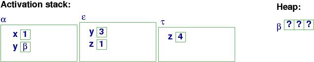
For the above program, when we reach point
(a), the machine looks like this:
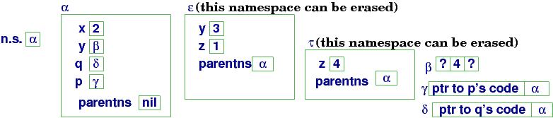
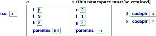
At (a):
The array is allocated
as a stand-alone object, and
y in namespace α is bound to handle
β, where the array's cells live.
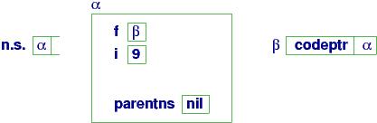
A declared procedure is saved in an object called a closure, that holds (at least) two items:
n.s. is the namespace stack. The top handle on n.s. is the handle to the variables that are visible to the currently executing command..
Finally, each namespace holds a field, parentns, which links to the namespace where nonlocal/``more global'' variables can be found. In our example, there are no ``more global'' variables to the main namespace, α. (But parentns becomes important in a moment!)
(IMPORTANT: The layout shown here is for an interpreted object language, like Smalltalk or Ruby or Python. Compiled object languages, like Java and C#, use a simpler layout, because the compiler pre-computes the closure and parentns linkages. In a later section, we examine the differences.)
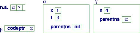
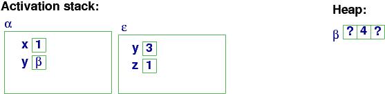
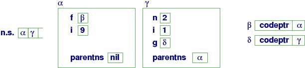
At point (a), the interpreter must compute q(3, x), so it first finds q's value, in namespace α --- it is handle δ. Next, x is found --- its value is 1. q's closure at δ is used to do these steps:
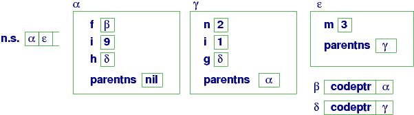
Here is the resulting storage configuration at procedure entry,
point (b):
At (b):
Within q's body, name lookups are done with
the top handle on n.s.
(ε), and if a name is
not found in ε, then ε's ``parent namespace'' (parentns)
α, is used, and so on.
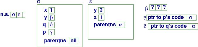
Procedure q calls p(x+y). The machine searches ε for p
with no luck. But a search of the parentns, α, locates p and
its value, γ, the handle to a closure. Next, the argument x+y is evaluated, finding x's value in α and y's in ε.
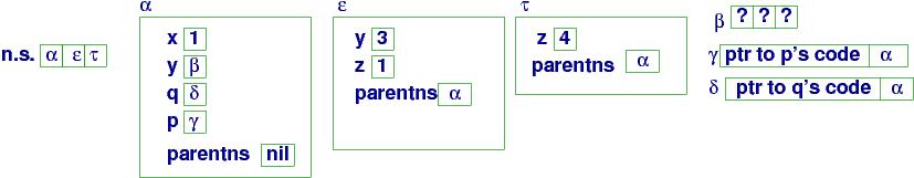
A new namespace, τ,
is allocated and initialized and τ is pushed onto
n.s..
p's
code (extracted from closure γ) computes with
τ. We arrive at (c) in the program:
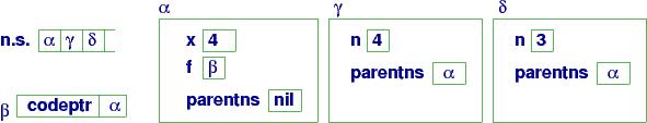
At (c):
Now p's code executes:
The assignment, y[x] = z, is correctly executed with array object
β, global variable x, and parameter z. (How are these values found,
starting from
τ?)
When procedure p finishes, its namespace handle is popped from the
namespace stack, n.s.,
giving this configuration
at (d):
At (d):
Namespace τ is an unneeded
object and can be erased from storage. Some programming languages
do this immediately; others wait and let the heap's garbage-collector
program erase the orphaned object.
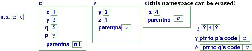
Procedure q finishes its work (x = z + 1) and returns, giving this final configuration:
At the end:
Important: Each time a procedure is called, a brand new namespace
is created for the call --- namespaces are never reused.
See the subsection that follows, "Recursively defined procedures", to see
why this implementation technique is the right one.
Here are two important concepts:
Exercise: Implement procedures with expression parameters within the interpreter for object languages. You must model the namespace stack and closure objects.
The beauty of the namespace stack is that it naturally supports
procedures that call themselves. For this little example,
which computes the factorial of 4,
===================================================

int x;
x = 1;
proc f(n) {
   if n > 0 {
      x = x * n;
      f(n - 1)
   }};
f(4)

===================================================
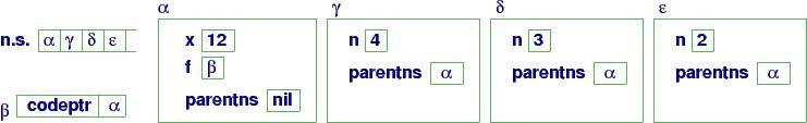
the storage configuration when f is entered the first time is
Namespaces for the main program and f's initial activation are
present in the heap. When the procedure calls (restarts) itself,
a fresh namespace is created for the fresh call:
The namespace stack now holds δ as the current namespace, and
references to n are resolved by
δ and references to global variable x are resolved
by the parent namespace, α, whose address is held
within namespace δ. (And this is why the
closure object for f remembers both a pointer to its code
as well as a pointer to the appropriate parent namespace.
This linkage from the current namespace to its parent namespace(s)
is sometimes called the static chain.)
Here is the state at the next call:
Eventually, n ``counts down'' to 0,
the sequence of self-calls complete, and the
namespaces pop one by one from the namespace stack,
leaving only α.
The diagrams for the examples match the implementation of interpreter-based object languages, like Smalltalk, Ruby, and Python.
Compiler-based object languages, like Java and C#, compile programs into target code that use computer storage differently --- the namespaces (frames) themselves for called procedures are allocated as the activation stack and when a procedure finishes, its namespace is immediately erased from the top of the stack.
For the earlier example, with procedures p and q, the compiled
Java/C# program would generate this memory layout at point (c):
and this layout at point (d), when p's call is finished:
Only the array is saved in the heap, and even the closures disappear.
There is no need for closure objects in Java/C# because the Java/C# compiler knows the addresses where the code for p and q reside. The Java/C# compiler also knows that the global variables for the two procedures will be found in the namespace at the bottom of the activation stack, because Java/C# use a C-style, simplistic nesting structure, where a command executes with one ``local namespace'' and one ``global namespace'' and that's it.
Now, the Java/C# approach works fine provided that a procedure never returns an
answer that is itself a procedure (or never allows a procedure's value
to be assigned to a global variable).
Java certainly disallows this, but C# provides a delegate definition
that can return and save procedures as values.
For example, if we write in C#,
delegate int IntToInt(int x)   // defines a "procedure type"
// assigns a closure's handle to var p:
IntToInt p = delegate(int i){i = i + 1; return i}
Console.WriteLine(p(2))       // prints 3
the C# compiler generates code that will construct a closure object
for p, exactly like the ones seen in the previous section, and the
call, p(2), operates like in the previous section.
Further, in an example like this:
delegate int IntToInt(int x);
class C { int i = 1;
          public void inc() { i = i + 1; }
          public IntToInt makeFun() {
              int j = i;
              return delegate(int k){ i = j + k; return j; }
          }
}
C ob = new C();
IntToInt f = ob.makeFun(); //  assigns a closure's handle to  f
ob.inc()                   //  resets  ob.i  to  2
Console.WriteLine(f(3));   //  resets  ob.i  to  4  (1 + 3)  and prints  1
the delegate value returned as the result
makes the C# compiler move the activation record for ob.makeFun()'s call
to the heap!
When an object language allows multiple levels of nonlocal variables or allows procedures to be assignable values, then the simplistic stack-heap storage layout shown in the previous picture fails. The virtual-machine model always works, however, and will be used later in this chapter in the section, ``Semantics of procedures with local variables.''
===================================================

int x;
int y[3];
void p(int x, int[] z) {
    z[x] = x;
}
 . . .
p(x+1, y)

===================================================
A compiler uses data types to allocate storage for variables and to check
for well-formedness properties, e.g.,
z[x] = x is a sensible assignment, because the types
of z and x are compatible.
Also, when the procedure is called, the compiler checks whether
the arguments that bind to the parameters match the types
listed with the parameter names.
In this way, the data types attached to parameter names assert a simplistic
precondition for a procedure.
Important: Once a variable is declared with a data type, then only values of that type can be assigned to that variable's location.
Some languages (e.g., Ocaml and Scala) let us
write typed procedures that take functions as arguments.
For example, procedure p in the following example
expects a function on ints and an int as its two arguments:
===================================================

int a;

fun f(int x) = x + 1;
// the data type of  f  is   int -> int
//   because it receives an int argument and returns an int answer

proc p((int -> int) q, int m) {
    a = q(m)
};

p(f, 3)  // this is a legal call and assigns  4  to  a

===================================================
The data type, int -> int, stands for a function that receives
an int argument and produces an int answer. This is why the call,
p(f, 3) is legal. Note that the call, p(a, 3) is illegal,
as is p(a + 1, 3) --- in both cases, the first argument is not a
parameterized function.
C# uses the delegate operator to define a function type:
delegate int IntArrowInt(int x);
int a;
int f(int x) { return x + 1; }
void p(IntArrowInt q, int m) { a = q(m); }
p(f, 3)
What is the type of a function that takes no arguments?
int a;
fun f() = a + 1;
//  f's  data type is  void -> int

a = 1;
a = f();   //  sets  a  to  2
We use void to mean ``no argument.''
Similarly,
void can mean ''no answer,'' like what a procedure
produces:
===================================================

int x;
proc f() {      // f  has type  void -> void
   x = x + 1
}

// g  requires another procedure as its argument:
proc g(void -> void  p) {
   // call  p  twice:
   p();
   p()
}

// h  requires a proc that requires a proc:
proc h(((void -> void) -> void) q) {
   q(f)
}
// these are all legal procedure calls:
f();
g(f);
h(g)

===================================================
As an exercise, recode these in C#.
The previous examples are not entirely artificial --- control
structures, like conditionals and loops, are commands that
take other commands as arguments. For example, a while-loop
is a procedure, defined like this:
===================================================

proc while(void -> boolean b, void -> void c) {
    if b() {
        c();
        while(b, c)
    }
}

===================================================
In this sense,
procedures that accept commands as arguments are
control structures --- you can even write your own control structures this way.
Here are two last interesting questions:
Some languages let you do this; it is called
a lambda abstraction. One looks like this:
lambda x : print x * 2
--- it is a procedure that doesn't have a name.
How do we use it? Well, we give it an argument, just
like we do when we call a procedure:
(lambda x : print x * 2)(4)
This command prints 8.
Or, we might write this:
(int -> void) p;
p = lambda x : print x * 2;
p(4)
where we declare p and later use it.
Now we realize that
proc d(x) {
    print x * 2
}
is the same thing as
d = lambda x : print x * 2;
Both are called by supplying an argument, e.g., d(4).
C# encodes a lambda abstraction like this, reusing the
delegate operator:
delegate void Comm(int x);
Comm d = delegate(int x) { print x * 2; }
d(4);
Consider this example, which can be written in a language like
Scheme, Lisp, or Python:
===================================================

def p(f, n) :
    if n > 2.0 :
        f(f, n/2.0)
    else :
        print n

===================================================
Parameter f must be a procedure-like abstract --- a control structure ---
because it takes control at f(f, n/2.0).
But we can call p like this: p(p, n). In this way,
p hands control to itself, like a loop does.
Now, what is the ``data type'' of p? Using the simplistic -> notation, we cannot write a (finite) type for p. This is a famous sticking point in data-type theory.
There are other kinds of patterns for parameters and arguments.
The first is called the keyword pattern,
because we label each argument to a procedure call with the name (``keyword'')
of the formal parameter to which it should bind.
For example,
===================================================

proc p(x, y) { ... };

p(y = 3, x = [2,3,5])  # 3 binds to parameter y,  [2,3,5] binds to x

===================================================
Procedure p expects two arguments, and the call provides
two arguments, but the keywords that are attached to the argument, not the order
of the arguments, defines the bindings. Keyword parameters are
useful in practice to making library procedures
easier to read and call.
Keywords in the declaration line of the procedure can set default
values for parameters. For example,
===================================================

proc p(x = [0,0,0], y = 0) = ...

===================================================
gives default values that are used if p is called with fewer than
a full set of arguments, e.g., p(y = 1) omits an argument for x
so the default applies. This use of defaults is helpful when you
call a library procedure that can receive many possible parameters,
but you wish to use the default values for all but a few.
Exercise: Implement keyword patterns with default values for expression parameters to procedures in the interpreter for object languages. (Hint: use dictionaries to collect the keywords and their default values.)
In addition to keyword patterns, there are structural patterns
which state the form of data structure that should be bound to a parameter.
For example, say that procedure p must receive an argument that is
an array (list) with 3 elements. We might define p
with a structural pattern, like this:
===================================================

proc p([first, second, third], y) =
    y = first + second + third;   // add the three elements
    print y

===================================================
Then the procedure might be called like this:
int[] r = [2,3,5];
p(r)
We might also have a pattern that says the array (list) has at least 3 elements:
proc p([first, second, third | rest], y) = ...
This form of pattern is found in Prolog. The rest part represents
a list that holds element 4 (if any) onwards.
Structural patterns are crucial to languages that let
us define our own data types with equations. In an earlier chapter,
we used
a data-type equation like this to define binary tree structures that hold
integers:
===================================================

datatype  bintree =  leaf of int | node of int * bintree * bintree

===================================================
Here is a bintree value; it is constructed with the keywords,
leaf and node:
mytree = node(2, leaf(3), node(5, leaf(7), leaf(11)))
We use structural patterns to write functions that process bintrees.
Here's one that sums all the integers
embedded in a tree:
===================================================

def sumTree(leaf(n)) = n
  | sumTree(node(n,t1,t2) = n + sumTree(t1) + sumTree(t2)

===================================================
The function
``splits'' its definition into two clauses, one for
each pattern of bintree argument. Of course, the above is merely
a cute replacement for
an if-command:
===================================================

def sumTree(tree) =
    if isinstance(tree, leaf(n)) :
        return n
    elif isinstance(tree, node(n,t1,t2)) :
        return  n + sumTree(t1) + sumTree(t2)

===================================================
When we call the function, e.g.,
sumTree(mytree), the structure of the argument is matched against
each of the two patterns in sumTree's definition to select the
appropriate computation:
===================================================

sumTree(mytree)

= sumTree(node(2, leaf(3), node(5, leaf(7), leaf(11))))

=> 2 + sumTree(leaf(3)) + sumTree(node(5, leaf(7), leaf(11))))

=> 2 + 3 + sumTree(node(5, leaf(7), leaf(11))))

=> 2 + 3 + (5 + sumTree(leaf(7)) + sumTree(leaf(11)))

=> 2 + 3 + (5 + 7 + 11)  =   28

===================================================
If you stare long enough
at the structural patterns for lists and trees,
you realize that an ``ordinary'' procedure definition, like
proc p(x,y,z) = ...
uses a structural pattern for a tuple data structure --- a tuple
of arguments. When we call p, we build a tuple argument to match
the tuple parameter pattern:
p(2, 3, [0,0,0])
Because of this coincidence, some languages let you write tuple
data structures as expressible values, like this:
int[] r = [0,0,0];
tup = (2, 3, r);   # tup names a tuple data structure
p(tup)             # or,  p tup
which calls p with its argument tuple.
In a similar fashion, keyword patterns are just a struct data
structure:
proc p(struct int x; int[] y end) = ...x...y...
 . . .
struct int x; int[] y end  mystruct;
mystruct.x = 2;
mystruct.y = [2,3,5];
p(mystruct)
This little example would be clearer if we named the
struct pattern,
like in C and Pascal:
type S = struct int x; int[] y end;

proc p(S) = ...
  . . .
S mystruct;
mystruct.x = 2;
mystruct.y = [2,3,5];
p(mystruct)
We develop this idea in the next chapter.
This concept was invented for the language, Algol60, a forerunner
of all modern assignment languages. It looks like this:
Say that we let
a command have private definitions by means of a
``begin-end'' block in the command syntax:
===================================================

C ::=  I = E  |  C1 ; C2  |  while E { C }  |  print I  |  I(E)
    |  begin D in C end

D ::=  int I = E  |  D1 ; D2  |  proc I1(I2) = C

===================================================
The new construction, begin D in C end, is called a command block.
Command blocks in Algol60 revolutionized the
way programmers thought about assembling programs, because
programmers started thinking of
programs as units that nest together.
(Algol60 also introduced the modern, structured form of if-then-else,
where the code for the then and else arms were command blocks!
Prior to Algol, conditionals were Fortran-like: ''IF test THEN GOTO labelnumber.'')
Here is a small example with a command block:
===================================================

int x = 1;  # (a)
begin
  int y = 3
in          # (b)
  y = y + x
  x = y + y # (c)
end;
# y  is not visible here  # (d)
print x  # prints 8

===================================================
The command block is an enclosed unit that owns a local (private) variable,
y, which cannot be referenced outside the block --- y is protected
from unauthorized use. Within the block both the ``global'' variable
x as well as the ``local'' variable y can be used.
Algol60 was designed to operate on a machine with a symbol table and a memory
(like the C-machine), but where both symbol table and memory are implemented
as stacks:
declared variables are allocated (pushed) on the memory
stack and are popped once they are no longer needed. Here is the
the execution of the above example:
At position (a):
symbol-table-stack = | x:0 |   // that is,  x  names location 0 in memory
memory = | 1 |

At position (b):
symbol-table-stack = | x:0 | y:1 |
memory = | 1 | 3 |

At position (c):
symbol-table-stack = | x:0 | y:1 |
memory = | 8 | 4 |

At position (d):
symbol-table-stack = | x:0 |
memory = | 8 |
The program's symbol table is also restructured as a stack that grows and
shrinks along with the memory.
The dual-stack setup helps a compiler and programmer precisely manage storage use.
In the 1960s, the Burroughs company built hardware computers with
stack memory. But it is so easy to emulate stacks with conventional
memory that the Burroughs machines disappeared from use after a few years.
These days, blocks are bonded to procedures, so that you
declare local variables along with parameters
when you write a procedure.
Here is a standard example:
===================================================

proc factorial(int n) {
begin
    int i = 0;
    int ans = 1;
in
    while i != n {
        i = i + 1;
        ans = ans * i
    };
    print ans
end }

===================================================
The body of factorial is a command block.
A call to factorial constructs one new namespace, which holds
parameter variable, n, as well as local variables,
i and ans. We see this in the next section.
We study an example that shows why the heap machine, with
its multiple namespaces, is needed for modern programming
languages. The example shows a procedure (impure function)
that owns a local procedure
and returns (a handle to) the local procedure as its answer.
(Almost every "modern" language can do this. C can't, and the original version of Java couldn't.)
===================================================

proc f(n) {
  begin var i = 1;
        proc g(m) {  # (d)
           print m + n + i
        }
  in  # (b)
      return g
  end
};
var i = 9;     # (a)
var h = f(2);  # (c)
h(3)           # (e)

===================================================
The call, f(2), returns the handle to a closure object that holds the code
for procedure g.
When the closure , now named h, is
called at h(3), the code within the closure object is activated,
and local variable m is assigned 3. Now, within g,
what is the value of n? Of i?
These should be found from
the local variables that were declared
in f's namespace when f was called earlier.
But f is no longer active.
How is this implemented? Not with a stack!
Here are a series of diagrams that show how this program executes.
When execution reaches program point (a), global names f and i
are declared and their values are saved in the main namespace, α:
At (a):
f's value is the handle to a closure object, which
holds (a pointer to) f's code and the address of f's parent namespace,
α.
The call, f(2), causes the closure at β to execute:
a new namespace, γ, is constructed and n has 2
in the namespace. The local variables, i and g, are added to
namespace γ, giving us the configuration at point (b):
At (b):
Variable g's value is a handle to another closure,
named δ,
and that closure uses γ as its parent link!
When f's code finishes,
δ is returned as the answer and is assigned to variable h
in α's namespace. Although the call to f has finished,
its namespace may not be erased, because it is needed by closure
δ:
At (c):
Next,
we call h(3), which activates the code attached
to closure δ and uses handle γ:
This creates namespace ε
to hold m = 3. The namespace
is used by the code body of g, and we reach point (d)
in the program:
At (d):
What names are visible at point (d)?
Entering namespace ε, we find
m. Following the parentns link,
γ, we find n, i, and g.
Following the link to the (grand)parent namespace,
we find f (but not i)
and h(!)
So, g's code can locate meanings for all of m, n, i, g, f, and h.
The collection of names visible from g's code is called g's
environment --- here, it is collected from three
distinct namespaces.
The program finishes by printing m + n + i (6) and popping the
activation stack.
The example shows that the namespaces constructed for procedure calls
cannot be automatically erased/popped when a procedure finishes, because data inside the namespace might be needed later.
Here is another example of this, using an assignment:
var p;
proc q(x): var y = 2;
           proc r(): print (x + y)  end;
           p = r;
end;
q(9);
p()  // executes  r's  code,  using  q's  x  and  y
A final remark: you cannot eliminate this "issue" by outlawing
procedures as values. When you have a language that uses handles
and when you can assign handles to variable names,
then you have this "issue." The original version of Java used some awkward restrictions
to try to avoid it, but in the end, Java was changed.
Exercise: Augment the interpreter for object languages to interpret procedures with local variables.
Each name in a program has a lifetime, or extent that is it saved in storage.
The collection of names whose scope cover a procedure's body is called the procedure's environment.
The abstraction principle: The phrases in any syntax domain may be named.
The parameterization principle: The phrases in any syntax domain may be arguments.
The qualification principle: The phrases in any syntax domain may own private (local) definitions.