Copyright © 2010 David Schmidt
Chapter 5:
Component extension by abstraction, parameterization, and qualification
- 5.1 The abstraction principle: Phrase structures can be named
- 5.1.1 Procedures
- 5.1.2 Functions
- 5.1.3 Other forms of abstracts
- 5.2 The parameterization principle: named phrases may accept arguments
- 5.2.1 Semantics of abstracts and parameters: Extent, scope, and namespaces
- 5.2.2 Data types for parameters
- 5.2.3 Patterns for parameters
- 5.3 The qualification principle: phrases may own private definitions
- 5.3.1 Semantics of procedures with local variables
- 5.4 Summary
Programs are usually
assembled from pieces, or components,
like functions, modules, and classes, and a programming language
must provide structures for defining and using components.
In this chapter, we see that the component mechanisms
in programming languages are
a product of several easy-to-state
principles first proposed by Robert Tennent of Queen's University,
Canada, in the 1970s. Tennent studied the origin of naming devices
for functions, procedures, modules, and classes and discovered
that they were based on one and the same theme. He later saw a similar
theme in the development of varieties of block structure.
Schmidt (your instructor at KSU) noted that Tennent's ideas also applied to
the forms of parameters that can be used with functions.
The results were the
abstraction, parameterization, and qualification principles
of language extension.
The three principles help us understand the structure, origins,
and semantics of component forms and they provide us
with advice as to how to add such forms to languages we
design.
In this chapter, we briefly survey
the principles and in subsequent chapters we apply them to understanding
and developing sophisticated languages.
5.1 The abstraction principle: Phrase structures can be named
The abstraction principle is stated as
-
The phrases in any semantically meaningful syntax domain may be
named.
This suggests, if our language has a syntax domain of commands, for example,
then we can name commands (they are procedures) and we can
execute (call) them by mentioning their names in any position
where a command might be used.
If our language has a syntax domain of expressions,
then we can name expressions (they are functions) and we can
call them by stating their names in any position where an expression
might be used.
Tennent titled the named phrases abstracts. That is,
procedures are ``command abstracts'' and functions are ``expression
abstracts'' and so on.
Indeed, every syntax domain of the language
might be nameable and callable.
This is the impact of the
abstraction principle. In the next chapter, we will see how concepts
like modules
and classes are immediate consequences of the abstraction
principle.
Here is a small example to get us thinking.
Say we have this core programming
language that computes on integers with assignments and loops:
===================================================

P : Program
E : Expression
C : Command
D : Declaration
I : Identifier
N : Numeral

P ::=  D ; C

E ::=  N  |  E1 + E2  |  E1 != E2  |  I

C ::=  I = E  |  C1 ; C2  |  while E { C }  |  print E

D ::=  int I  |  D1 ; D2

N ::=  0 | 1 | 2 | ...

I ::=  alphanumeric strings

===================================================
The language's denotable values are integer variables;
the storable and expressible values are just integers.
The abstraction principle says we can name
the constructions in the various syntax domains.
Let's start with commands:
5.1.1 Procedures
If we give names to commands,
then we have procedures; the language extends to this:
===================================================

D ::=  int I  |  D1 ; D2  |  proc I = C end

C ::=  I = E  |  C1 ; C2  |  while E { C }  |  print E  |  I()

===================================================
There is a new declaration construction, proc I = C, which makes I
name command C. (Other possible forms of syntax are
proc I() { C } or def I(): C or
void I() { C }, but the main point is that I names C.)
Is identifier I a variable, that is, can its value vary?
(In some languages, yes, in others, no.
We return to this question in a bit.)
Now, an identifier in the language can denote a command as well as
an int variable.
To reference (call) a procedure, we state its name wherever a command
can appear; this is why we see
C ::= . . . | I()
in the syntax for commands. (Perhaps you prefer call I or just
I for the syntax --- take your pick.)
Here is an example that uses a procedure to
compute the factorial of a nonnegative int, n:
===================================================

int i;
int ans;
int n;
proc factorial =
    i = 0;
    ans = 1;
    while i != n {
        i = i + 1;
        ans = ans * i
    }
    end;
n = 4;
factorial();
print ans

===================================================
The classic semantics of a procedure says that the procedure's
commands (its body) are executed with the current
value of storage at the position
where the procedure is
called. The example program executes this sequence of
commands:
n = 4
factorial() +--> # factorial's body commences:
                 i = 0
                 ans = 1
                 while i != n {
                    i = i + 1
                    ans = ans * i }
  < -----------+
print ans
The program executes as if the procedure's body is copied in place
of its calling command --- this is the ``copy rule'' semantics
of calls, mentioned in earlier chapters. A computer implements
a copy-rule-style semantics with an instruction counter and
stack of namespaces (activation
records), as we see later in this Chapter.
Given that a procedure is declared like a variable is declared,
can we assign to a procedure like we do a variable?
For example, are we allowed to update procedure code, like this?
===================================================

int i;
proc p =  i = i + 1  end;
i = 2;
p = (i = i * i)

===================================================
If yes, then p denotes a variable command, and commands are
storable (updatable)
values. If no, then it means that p denotes a constant command
that cannot be altered once it is named by p.
(What does your favorite language let you do?)
In the example, with factorial, the procedure references
variables, i, ans, and n. This is justifiable, since the
sequential control structure, D1 ; D2, elaborates the declarations
from left to right, processing D1 first and making it
available in D2. A more delicate question
is whether factorial might call itself, like this:
int i;
int ans;
int n;
proc factorial =
      if i != n {
          i = i + 1;
          ans = ans * i;
          factorial()
      }
      end;
print factorial()
This is normally allowed. Here is an example execution:
===================================================

n = 3;
i = 1;
ans = 1;
factorial() ---> # In storage,  i == 1  and  ans == 1
                 if i != n
                 i = i + 1 ;
                 ans = ans * i ;
                 factorial() ---> # Now,  i == 2,  ans == 2
                                    if i != n
                                    i = i + 1 ;
                                    ans = ans * i ;
                                    factorial() ----> # i == 3, ans == 6
                                                      if i != n
                                    <-----------------+
                 <------------------+
<----------------+
# In storage,  n == 3,  i == 3,  and  ans == 6

===================================================
We will study the implementation of procedures in a later section,
once we add parameters to them.
If we can name commands, then we might try naming expressions
as well; these are called (pure) functions:
===================================================

E ::=  N  |  E1 + E2  |  E1 != E2  |  I  |  I()

D ::=  int I  |  D1 ; D2  |  proc I = C  |  fun I = E

===================================================
We will use I() to represent a function call, to distinguish
it from I, the construction for variable lookup.
Here is a small example:
===================================================

int i;
i = 0;
fun f = (i + i) + 1;
i = i + 1;
i = f() + f() - i

===================================================
Immediately we encounter a serious question:
What is the ``value''
of f immediately after the declaration, fun f = ...?
There are actually two possibilites:
-
f's value is 1, because
i = 0;
fun f = (i + i) + 1;
and because
(i + i) + 1 computes to 0 + 0 + 1 == 1.
This would mean that the later use of f in
i = f() + f() - i
updates i to
f() + f() - 1, which equals 1 + 1 - 1 which equals 1.
This is called eager evaluation of function f,
because the function's body code is computed immediately, when the function
is defined!
Does your favorite language use functions in this way?
Probably not! If you wanted f to be eagerly evaluated, you
would have written int f = (i + i) + 1 instead, right?
-
Instead, f's value is the expression --- the code ---
(i + i) + 1. This means, when f() is called,
its body is evaluated only then. In the above program,
the commands that execute proceed like this:
1. allocate cell for  i
2. assign  0  to  i
3. assign code to  f
4. assign the value of  i+1  to  i
5a. call function  f,  that is, execute the expression it names
5b. call function  f,  that is, execute the expression it names
5c. add  the answers from  5a and 5b, subtract  i's  value, and assign to  i
that is,
# allocate cell for  i
i = 0
# save  f's code
i = i + 1
i = ((i + i) + 1) + ((i + i) + 1) - i   # the calls to  f  are expanded
                                        # and  i  is updated to  5
This matches the ``copy-rule semantics'' that we used to understand
procedure calles. It is also known
as lazy evaluation, because f's code is evaluated
only when it is needed.
The copy-rule semantics makes clear that
functions are a ``shorthand'' for remembering commonly used
expressions, saving us the trouble of copying and pasting text.
To eliminate confusion about eager and lazy evaluation,
most languages
use this syntax for function definition:
fun f() { E }
The () can be read as an ``empty argument tuple,''
and the syntax nicely matches the syntax, f(), that we use
to call the function.
The function definition
no longer looks like an assignment!
This story also suggest why procedures are typically defined
with the () notation also, even when a procedure requires no
parameters, e.g.,
proc p() { x = x + 1 }
Later, we will see how to implement function definition and function call.
Functions can be surprisingly powerful.
If the syntax of Expression includes a conditional construct, that is,
E ::= ... | if E1 then E2 else E3
then we can use it along with recursion (self-call) to implement
recurrence relations. Here is the mathematical specification
of factorial:
0! == 1
n! == (n - 1)! * n,   for integers  n > 0
We use the spec to write this pure function (with one parameter):
fun fac(n) =  if n == 0 then  1
              else  n * fac(n-1)
Based on the earlier examples with copy-rule semantics,
you can
calculate that
===================================================

fac(3) => n = 3
          if n == 0 then  1
          else  n * fac(n-1)

       =  3 * fac(3-1)  =>  n = 2
                            if n == 0 then  1
                            else  n * fac(n-1)

                        =   2 * fac(2-1)  =>  n = 1
                                              if n == 0 then  1
                                              else  n * fac(n-1)

                                          =   1 * fac(0)  =>  n = 0
                                                              if n == 0 then  1
                                                              else  fac(n-1) * n

                                                           =>  1
                                          =   1 * 1 = 1

                        =  2 * 1 = 2

       =  3 * 2  = 6
= 6

===================================================
Most general-purpose languages omit pure functions
in favor of procedures that quit with a return E command.
Here is factorial, written as a procedure that returns an answer. Notice how
the loop updates variable n's value as it proceeds:
===================================================

int n;
proc fac() =
    ans = 1;
    while n != 0 {
        ans = ans * n
        n = n - 1 };
    return ans
end;
n = 4;
total = n + fac() + n   # total is assigned  4 + 24 + 0 (!)

===================================================
Many people call this form of abstract a ``function,'' but more
precisely, it is a procedure that returns an answer.
Since the ``procedure-function'' contains
commands, it can change variables like n from
4 to 0,
so that the name, n, yields two different numbers in the
expression, n + fac() + n.
In practice, the standard, benign use of a procedure-function is within
a simple assignment of this form:
answer = fac()
5.1.3 Other forms of abstracts
We can go further than procedures and functions --- looking
at the core language definition, we might consider Declaration abstracts and
Numeral abstracts and even Identifier abstracts!
Declaration abstracts are very important --- they are commonly known
as
modules and will be studied in detail in the next chapter.
Numeral abstracts are
sometimes called
final variables or consts.
Does your favorite language have these?
Identifier abstracts are called aliases. An alias
copies the address of one variable as the address of another.
In an object language or a language that has pointer variables,
alias abstracts add no new facility.
5.2 The parameterization principle: named phrases may accept arguments
The abstraction principle shows how we can name phrases.
It makes sense that we can use parameter names
with the named phrases themselves. This is the
principle of parameterization:
-
The phrases in any semantically meaningful syntax domain may be arguments to
abstracts.
The best known example of the parameterization principle is
the use of expression parameters to procedures ---
any phrase that is an expression can be an argument that is assigned
to a procedure's parameter. For the example language
with procedures,
we can allow expressions as parameters:
===================================================

E ::=  N  |  E1 + E2  |  E1 != E2  |  I

C ::=  I = E  |  C1 ; C2  |  while E { C }  |  print I  |  I(E)

D ::=  int I  |  D1 ; D2  |  proc I1(I2) { C }

===================================================
The procedure is defined as proc I1(I2) { C },
and the procedure must be called with an expression, E, that is assigned
to parameter I2, like this: I1(E).
The syntax is not limited to exactly one parameter; you can have zero
or many parameters, like this:
C ::=  I = E  |  C1 ; C2  |  while E { C }  |  print I  |  I(E*)

D ::=  int I  |  D1 ; D2  |  proc I1(I*) { C }
where E* (also I*) means zero or more of E (I), separated
by commas.
Within the procedure, the parameter's value is used
by referring to it by its name, just like we call a function
by referring to it by name.
Here again is a factorial procedure with a parameter:
===================================================

int ans;
proc fact(n) {
    ans = 1
    while n != 0 {
        ans = ans * n;
        n = n - 1
    }};
int x;
x = 2;
fact(x + x);
print ans

===================================================
When fact is called, x + x is bound
to the parameter name, n. How is this done?
-
Most modern languages use ``assignment binding,'' also known as
call by value --- the assignment,
n = x + x, is assembled and executed as the first command
of the called procedure. The program executes like this:
x = 2
fact(x + x)  +--->  n = x + x
                    ans = 1
                    while n != 0 {
                      ans = ans * n
                      n = n - 1 }
             <----+
# at this point,  variable  n  no longer exists!
# but  ans  and  x  still do....
-
Some languages (e.g., C#) offer another form of parameter binding, call by
reference. Here, the formal parameter is a ``pointer''
to the cell named by the argument, which must be a variable.
For the above example,
int ans;
proc fact(n) {  # say that  n  is call-by-reference
    ans = 1
    while n != 0 {
        ans = ans * n;
        n = n - 1
    }};
int x;
x = 2;
fact(x);
print ans
the semantics of the call looks like this, where we use the & and
* operators of C to denote ''location of'' and ''contents of'',
respectively:
int x;
x = 2;
fact(x)  +----> n = &x   # n is assigned x's location
                ans = 1
                while *n != 0 {
                  ans = ans * (*n);
                  *n = *n - 1
         <----+
print ans
Correspondences: eager and lazy evaluation of parameters
Since call by value is the most common form of parameter binding for
expressions,
many people do not think further about other options.
Well, think about this: There seems to be a ``correspondence''
in the way we define functions (expression abstracts)
and expression parameters. In both cases, an identifier
is equated to an expression. But wait --- when we define a function, n,
like
fun n() =
    x + x
we do not evaluate the body, x + x, until
the function is called.
On the other hand, when we define a parameter, n, like we did above:
proc fact(n) = ...
   ...
fact(x + x)
we evaluate the ``body,'' x + x, immediately
and do not wait to see if n is used or not.
When a evaluation is delayed, as it is for function
n, we say that n is lazily evaluated. When the binding
is evaluated as soon as possible, as it is for argument n,
we say that n is eagerly evaluated.
Haskell is the best known language that uses lazy evaluation for
all its abstract forms and all its parameter forms. All other
languages have more complex combinations: typically, abstracts are
evaluated lazily and arguments are evaluated eagerly.
Make certain you understand the evaluation
strategies for the language you use.
Other parameter forms
Other phrase forms can be parameters.
For the example language, we already have procedures, that is,
we already know how to name commands. It seems that
we already have in place the semantic machinery
to use commands as parameters ``for free,''
since a command parameter names a command.
Here is the little language with procedures that use command parameters:
===================================================

C ::=  I := E  |  C1 ; C2  |  while E { C }  |  print I  |  I(C)  |  I

D ::=  int I  |  D1 ; D2  |  proc I1(I2) { C }

===================================================
(If we develop this example further, we must ask the question
whether eager or lazy evaluation should be used for command parameters!)
The example suggests that the
notion of naming is
the same, whether we name a command abstract or
a command parameter.
When you pass an event-handler procedure as an argument to a set-up
method for a widget in a graphics library, you are using a command
parameter.
In the Python language, procedure names are variables, just like
integer variables, and all abstracts are evaluated lazily and
all parameter arguments are evaluated eagerly. Here is an interesting
example:
===================================================

x = 2

def p():     # p is assigned the handle (pointer) to an object that holds the proc code
  x = x + 1

def q(z):
  z()

r = p        # r is assigned p's handle
p = x        # p is updated to int 2
q(r)         # calls  q  with the handle
print x      # prints  3  (why?)

===================================================
Because p is a variable, the def command is actually
an assignment to p of a handle to a closure, which is an object that holds code.
So, r is assigned the handle to p's closure.
Even though p is updated by p = x, the call,
q(r), will assign the handle to parameter z,
and the the closure is called at z(). This causes x = x + 1
to execute. We study the implementation in the next section.
5.2.1 Semantics of abstracts and parameters: Extent, scope, and namespaces
We now study how an interpreter gives semantics to
abstracts and parameters. We will focus on adding procedures
with expression parameters to the interpreter for object languages.
Here is an interesting example, where procedure p uses
a parameter name that is the same as a
name already declared:
===================================================

int x;
int[3] y;
proc p(x, z) {
    # (b)
    z = x + y[1];
    y[x] = z
    # (c)
};
x = 1;
y[1] = 5;
# (a)
p(x + x, 0);
# (d)
print x;

===================================================
The program's global variables are integer variable x and array y.
These names, along with p, will be saved in the program's environment
(namespace). But when p is called, it uses a different
namespace, which holds parameter names x and z.
But array y is also visible to p's body, too!
We will implement this situation with a new data structure:
a namespace stack, which remembers the namespaces
in use
in the program. (Sometimes, the namespace
stack is called the activation-record stack
or the dynamic chain.)
For the above program, after the declarations for x, y, and p
are saved, and the two assignments are executed, we reach
point (a). The intepreter's data structures look like this:
At (a):
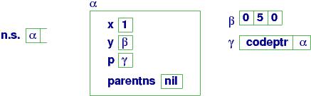
n.s. is the namespace stack.
The namespace stack remembers that the namespace at address
α holds the declarations for the main program:
x holds an int,
y holds the handle, β, to an array object,
and p holds the handle, γ, to a closure object.
The closure holds
a pointer to p's code and also the address of the parent (global) namespace
that p's body will use to look up nonlocal variables.
At point (a), the interpreter must compute
p(x + x, 0), so it first computes x's value. The interpreter consults
the top of the namespace stack to find α, where
x is found in the namespace --- its value is 1. The interpreter computes the two
arguments, 2 and 0.
Next, p is located, also in the namespace at α,
and its closure at γ is used to do these steps:
-
A new namespace object is allocated in the heap.
Say that its handle is δ.
-
Variables x and z are allocated within the new namespace
and are assigned 2 and 0, respectively.
Also, the α handle extracted from the closure is assigned
to the parentns variable in the new namespace.
-
The handle, δ, is pushed onto the namespace stack.
It becomes the ``current namespace'' in use, the one used by p's
code.
Here is the resulting storage configuration at procedure entry,
point (b):
At (b):
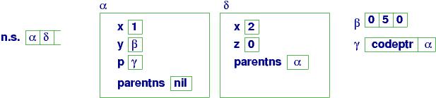
The new namespace, δ, holds variables x and z,
and the namespace is topmost on the namespace stack.
Within p's body, all references to x and z are handled
by this namespace. References to y (and p) are handled
by first searching namespace δ and since the names are
not found there, searching δ's ``parent namespace''
(see the cell, parentns, in δ), &alpha.
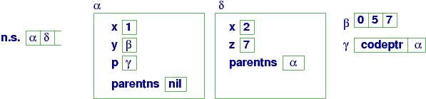
When the function is ready to finish, at point (c),
the updates on the namespaces
and array object β are accomplished:
At (c):
When procedure p finishes, its namespace handle is popped from the
namespace stack,
giving this configuration
at point (d):
At (d):
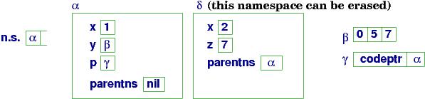
The computer resumes executing the commands in the main program.
Namespace δ is now an unneeded
object and can be erased from storage. Some programming languages
do this immediately; others wait and let the heap's garbage-collector
program erase the orphaned object.
Scope and extent
Here are two important concepts:
-
Each name in a program has a scope,
which is the portion of the program
where the name is visible.
In the above example program,
the scope of parameter z is
just the body of procedure p, and the scope of y is the
entire program. The scope of the first, outer declaration of x
is the entire program except for procedure p.
-
Each name in a program has a lifetime, or extent,
which is the part of the program's exection when the name and its value
are saved in storage.
In the previous example, the extent of parameter x is
the time during which a call of p executes. (When p finishes,
the namespace holding x is erased.)
The extent of global variable x is the entire time from when
x is declared until the program stops. Even when x is invisible
(e.g., when p's body executes), the global variable is present in
heap storage.
Exercise: Implement procedures with expression parameters
within the interpreter for object languages.
You must model the namespace stack and closure objects.
Recursively defined procedures
The beauty of the namespace stack is that it naturally supports
procedures that call themselves. For this little example,
which computes the factorial of 4,
===================================================

int x;
x = 1;
proc f(n) {
   if n > 0 {
      x = x * n;
      f(n - 1)   # (b)
   }};
f(4)   # (a)

===================================================
the storage configuration when f is started the first time is
Namespaces for the main program and f's initial activation are
present in the heap. When the procedure calls (restarts) itself,
a fresh namespace is created for the fresh call:
The namespace stack now holds δ as the current namespace, and
references to n are resolved by
δ and references to global variable x are resolved
by the parent namespace, α, whose address is held
within namespace δ. (And this is why the
closure object for f remembers both a pointer to its code
as well as a pointer to the appropriate parent namespace.
This linkage from the current namespace to its parent namespace(s)
is sometimes called the static chain.)
Here is the state at the next call:
Eventually, n ``counts down'' to 0,
the sequence of self-calls complete, and the
namespaces pop one by one from the namespace stack,
leaving only α.
5.2.2 Data types for parameters
In the first example in the previous section, both
integer and array parameters were manipulated by procedure p.
It would be helpful to label p's parameters with appropriate information,
perhaps like this:
===================================================

int x;
int y;
proc p(int x, int[] z) {
    z[x] = y;
    y = x + z[0]
}

===================================================
With the data types labelling the parameters, we can check
p's body for basic well-formedness properties, e.g.,
z[x] = y is a sensible assignment, because the types
of z, x, and y are compatible.
Also, when the procedure is called, we can check whether
the arguments that bind to the parameters match the types
listed with the parameter names.
In this way, data types attached to parameter names assert a simplistic
precondition for a procedure.
Important: Once a variable is declared
with a data type, then only values of that type can be assigned to that
variable's location.
A compiler, say, for C or Java, uses the data types to identify
possible mismatches of arguments to parameters. This saves debugging time.
Some languages (e.g., Ocaml) let us
write typed procedures that take functions as arguments.
For example, procedure p in the following example
expects a function on ints and an int as its two arguments:
===================================================

int a;

fun f(int x) = x + 1;
// the data type of  f  is   int -> int
//   because it receives an int argument and returns an int answer

proc p((int -> int) q, int m) {
    a = q(m)
};

p(f, 3)  // this is a legal call and assigns  4  to  a

===================================================
The data type, int -> int, stands for a function that receives
an int argument and produces an int answer. This is why the call,
p(f, 3) is legal. Note that the call, p(a, 3) is illegal,
as is p(a + 1, 3) --- in both cases, the first argument is not a
parameterized function.
What is the type of a function that takes no arguments?
int a;
fun f() = a + 1;
//  f's  data type is  void -> int

a = 1;
a = f();   //  sets  a  to  2
We use void to mean ``no argument.''
In a similar way,
void can be used to mean ''no answer,'' like what a procedure
produces.
In the example that follows below, procedure f has type void -> void,
and procedure g requires another
procedure as its argument, and h requires for its
argument a procedure that requires a procedure:
===================================================

int x;
proc f() {
   x = x + 1
}
// f  has type  void -> void

// g  requires another procedure as its argument:
proc g(void -> void  p) {
   // call  p  twice:
   p();
   p()
}

// h  requires a proc that requires a proc:
proc h(((void -> void) -> void) q) {
   q(f)
}
// these are all legal procedure calls:
f();
g(f);
h(g)

===================================================
The previous examples are not entirely artificial --- control
structures, like conditionals and loops, are commands that
take other commands as arguments. For example, a while-loop
is a procedure, defined like this:
===================================================

proc while(void -> boolean b, void -> void c) {
    if b() {
        c();
        while(b, c)
    }
}

===================================================
In this sense,
procedures that accept commands as arguments are
control structures --- you can even write your own control structures this way.
Here are two last interesting questions:
-
Can we write an expression (not a function or proc
definition) of type, say, int -> void?
Some languages let you do this; it is called
a lambda abstraction. One looks like this:
lambda x : print x * 2
--- it is a procedure that doesn't have a name.
How do we use it? Well, we give it an argument, just
like we do when we call a procedure:
(lambda x : print x * 2)(4)
This command prints 8.
Or, we might write this:
(int -> void) p;
p = lambda x : print x * 2;
p(4)
where we declare p and later use it.
Now we realize that
proc d(x) {
    print x * 2
}
is the same thing as
d = lambda x : print x * 2;
Both are called by supplying an argument, e.g., d(4).
-
Can a procedure take itself as an argument?
Consider this example, which can be written in a language like
Scheme, Lisp, or Python:
===================================================

def p(f, n) :
    if n > 2.0 :
        f(f, n/2.0)
    else :
        print n

===================================================
Parameter f must be a procedure-like abstract --- a control structure ---
because it takes control at f(f, n/2.0).
But we can call p like this: p(p, n). In this way,
p hands control to itself, like a loop does.
Now, what is the ``data type'' of p? Using the simplistic
-> notation, we cannot write a (finite) type for p.
This is a famous sticking point in data-type theory.
5.2.3 Patterns for parameters
A data type attached to a parameter name
restricts the range of values that might be bound to
the parameter. The data type is a kind of ``pattern''
that the argument must match.
Keyword patterns
There are other kinds of patterns for parameters and arguments.
The first is called the keyword pattern,
because we label each argument to a procedure call with the name (``keyword'')
of the formal parameter to which it should bind.
For example,
===================================================

proc p(x, y) { ... };

p(y = 3, x = [2,3,5])  # 3 binds to parameter y,  [2,3,5] binds to x

===================================================
Procedure p expects two arguments, and the call provides
two arguments, but the keywords that are attached to the argument, not the order
of the arguments, defines the bindings. Keyword parameters are
useful in practice to making library procedures
easier to read and call.
Keywords in the declaration line of the procedure can set default
values for parameters. For example,
===================================================

proc p(x = [0,0,0], y = 0) = ...

===================================================
gives default values that are used if p is called with fewer than
a full set of arguments, e.g., p(y = 1) omits an argument for x
so the default applies. This use of defaults is helpful when you
call a library procedure that can receive many possible parameters,
but you wish to use the default values for all but a few.
Exercise: Implement keyword patterns with
default values for expression
parameters to procedures in the interpreter for object languages.
(Hint: use dictionaries to collect the keywords and their default
values.)
Structural patterns
In addition to keyword patterns, there are structural patterns
which state the form of data structure that should be bound to a parameter.
For example, say that procedure p must receive an argument that is
an array (list) with 3 elements. We might define p
with a structural pattern, like this:
===================================================

proc p([first, second, third], y) =
    y = first + second + third;   // add the three elements
    print y

===================================================
Then the procedure might be called like this:
int[] r = [2,3,5];
p(r)
We might also have a pattern that says the array (list) has at least 3 elements:
proc p([first, second, third | rest], y) = ...
This form of pattern is found in Prolog. The rest part represents
a list that holds element 4 (if any) onwards.
Structural patterns are crucial to languages that let
us define our own data types with equations. In an earlier chapter,
we used
a data-type equation like this to define binary tree structures that hold
integers:
===================================================

datatype  bintree =  leaf of int | node of int * bintree * bintree

===================================================
Here is a bintree value; it is constructed with the keywords,
leaf and node:
mytree = node(2, leaf(3), node(5, leaf(7), leaf(11)))
We use structural patterns to write functions that process bintrees.
Here's one that sums all the integers
embedded in a tree:
===================================================

def sumTree(leaf(n)) = n
  | sumTree(node(n,t1,t2) = n + sumTree(t1) + sumTree(t2)

===================================================
The function
``splits'' its definition into two clauses, one for
each pattern of bintree argument. Of course, the above is merely
a cute replacement for
an if-command:
===================================================

def sumTree(tree) =
    if isinstance(tree, leaf(n)) :
        return n
    elif isinstance(tree, node(n,t1,t2)) :
        return  n + sumTree(t1) + sumTree(t2)

===================================================
When we call the function, e.g.,
sumTree(mytree), the structure of the argument is matched against
each of the two patterns in sumTree's definition to select the
appropriate computation:
===================================================

sumTree(mytree)

= sumTree(node(2, leaf(3), node(5, leaf(7), leaf(11))))

=> 2 + sumTree(leaf(3)) + sumTree(node(5, leaf(7), leaf(11))))

=> 2 + 3 + sumTree(node(5, leaf(7), leaf(11))))

=> 2 + 3 + (5 + sumTree(leaf(7)) + sumTree(leaf(11)))

=> 2 + 3 + (5 + 7 + 11)  =   28

===================================================
Correspondences
If you stare long enough
at the structural patterns for lists and trees,
you realize that an ``ordinary'' procedure definition, like
proc p(x,y,z) = ...
uses a structural pattern for a tuple data structure --- a tuple
of arguments. When we call p, we build a tuple argument to match
the tuple parameter pattern:
p(2, 3, [0,0,0])
Because of this coincidence, some languages let you write tuple
data structures as expressible values, like this:
int[] r = [0,0,0];
tup = (2, 3, r);   # tup names a tuple data structure
p(tup)             # or,  p tup
which calls p with its argument tuple.
In a similar fashion, keyword patterns are just a struct data
structure:
proc p(struct int x; int[] y end) = ...x...y...
 . . .
struct int x; int[] y end  mystruct;
mystruct.x = 2;
mystruct.y = [2,3,5];
p(mystruct)
This little example would be clearer if we named the
struct pattern,
like in C and Pascal:
type S = struct int x; int[] y end;

proc p(S) = ...
  . . .
S mystruct;
mystruct.x = 2;
mystruct.y = [2,3,5];
p(mystruct)
We develop this idea in the next chapter.
5.3 The qualification principle: phrases may own private definitions
A procedure's
parameter names are local or ``private'' variables
in the sense that only the procedures's body can use the parameter
names; outside the function, the parameter names are not visible.
(See the diagrams in the previous section that showed how namespaces
are used.)
The concept of local variable suggests a
third, powerful principle, the qualification principle:
-
The phrases in any semantically meaningful syntax domain may own
private (local) definitions.
A private definition is just that --- a definition that
is used by one phrase and not the entire program. This principle
is sometimes called ``hiding'' or ``encapsulation.''
We will make important use of the qualification principle in
upcoming chapters, but here is one instance that illustrates
key concepts: say that we
allow a command to have private definitions; we add a
``begin-end'' block to the command syntax:
===================================================

C ::=  I = E  |  C1 ; C2  |  while E { C }  |  print I  |  I(E)
    |  begin D in C end

D ::=  int I = E  |  D1 ; D2  |  proc I1(I2) = C

===================================================
The new construction, begin D in C end, is called a command block.
Command blocks first appeared in Algol60 and they revolutionized the
way programmers thought about structuring programs, because the
blocks caused programmers
to think of programs as
units that connect or nest together.
Here is a small example with a command block:
===================================================

int x = 0;
begin
  int y = 1
in
  y = y + x
  x = y + y
end;
# y  is not visible here
print x  # prints  2

===================================================
The command block is an enclosed unit that owns a local (private) variable,
y, which cannot be referenced outside the block --- y is protected
from unauthorized use. Within the block both the ``global'' variable
x as well as the ``local'' variable y can be used.
Here is a second example that shows how a local variable can use
the same name as a global variable:
===================================================

int x = 0;
int y = 9;
begin
  int y = x + 1
in
  x = y + y
  print y   // prints 2
end ;
print y     // prints 9

===================================================
Inside the command block, the local variable y is visible, but
the global is not. After the block finishes, the global y is visible
but the local is not.
Here is a variation on the previous example:
===================================================

int x = 1;
int y = x;
begin
  int x = 2;
  int y = y + x  // what value is computed for  y + x ?  Or is it an error ?
in
  print y
end

===================================================
There are multiple possible answers to the question asked in the code.
What do you think? We would have to study the semantics of the language
to know for certain.
Local variables in a block behave the same as parameter variables
inside a procedure. When a block is entered, it is like entering
the body of a called procedure --- local variables are declared within
a new namespace, created for the block. When the block finishes,
it is like a procedure finishing. The laws for scope and extent
for local variables are the same as they are for parameters.
Because parameter-argument bindings and local variables are ``the same,'' almost
all languages let you declare local variables along with parameters
when you write a procedure.
Here is a standard example:
===================================================

proc factorial(n) {
begin
    int i = 0;
    int ans = 1;
in
    while i != n {
        i = i + 1;
        ans = ans * i
    };
    print ans
end }

===================================================
The body of factorial is a command block.
A call to factorial would construct one new namespace, which holds
the procedure's parameter variable, n, as well as its local variables,
i and ans. We see this in the next section.
Static and dynamic scoping
Here is a slightly tricky question about the scope of a global variable:
What does this program print?
===================================================

int i = 0;
proc p() {
   i = i + 1
};

begin
  int i = 9
in
  p();           // which  i  is updated by  p ?
  print i        // does it print  9  or  10 ?
end;
p();             // which  i  is updated by  p ?
print i          // does it print  1  or  2 ?

===================================================
If p is statically scoped, the global variable i that appears in
p's scope when p is declared is the one that is
updated when p is called.
But the call, p(), within the block has another
variable i --- maybe this one should
be updated instead? In the latter case, p is dynamically
scoped. Dynamic scoping is easier to implement than static
scoping,
but look again
at p's declaration, isolated from its use:
int i = 0;
proc p() {
     i = i + 1
};
Dynamic scoping easily
misleads us about what p does.
For this reason, modern programming languages implement
static scoping with procedures.
When you learn a new language,
always learn, first thing, if its procedures operate with static
or dynamic scoping.
5.3.1 Semantics of procedures with local variables
We study an example that shows procedures with local
variables and static scoping. This example contains a procedure
that owns a local procedure
and returns (a handle to) the local procedure as its answer:
===================================================

proc f(n) {
  begin int i;
        proc g(m) {
           # (d)
           print m + n + i
        }
  in
     i = 1;
     # (b)
     return g
  end
};
int i = 9;
# (a)
h = f(2);
# (c)
h(3)
# (e)

===================================================
The call, f(2), returns a closure object that holds the code
for procedure g.
When the closure object, now named h, is
called at h(3), the code within the closure object is activated,
and m is assigned 3. When the closure object executes,
what is the value of n? Of i?
Static scoping says that the n and the i referenced inside g's code must
be the local variables that were
saved within f's namespace.
But f is no longer active.
How is this implemented?
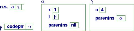
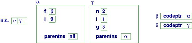
Here are a series of diagrams that show storage while this program executes.
They show how namespaces implement static scoping.
When execution reaches program point (a), global names f and i
are declared and their values are saved in the main namespace, α:
At (a):
Note that f's value is the handle to a closure object, which
holds a pointer to f's code and the address of f's parent namespace,
α.
The call, f(2), causes the closure at β to execute:
a new namespace, γ, is constructed and n has int value 2
in the namespace. The local variables, i and g, are added to
namespace γ, giving us configuration at point (b):
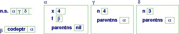
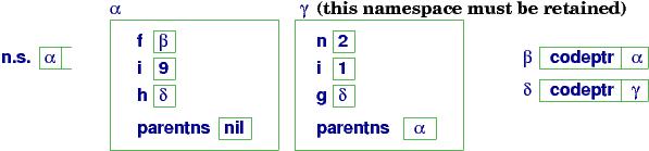
At (b):
Notice that local variable g's value is a handle to another closure,
named δ,
and notice that the closure contains γ.
When f's code finishes,
g's value, δ --- a handle --- is returned as the answer and is assigned to variable h
in α's namespace. Although the call to f has finished,
its namespace may not be erased, because it is needed by closure
δ, which is h's value. Indeed, at point (c),
we are ready to call h(3), which will activate the code attached
to closure δ:
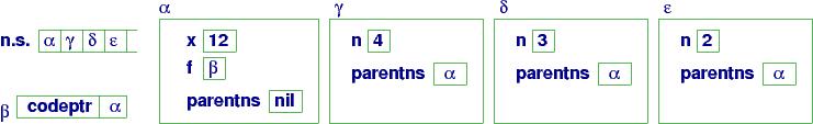
At (c):
When the call h(3) commences, this causes namespace ε
to be created to hold the assignment of m to 3. The namespace
is used by the body of function g, and we reach point (d)
in the program:
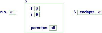
At (d):
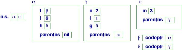
Now, what what names are visible at point (d)?
Entering namespace ε, we find a denotation for
m. Following the link to the parent namespace,
γ, we find meanings for n, i, and g.
Following the link to the (grand)parent namespace,
we find meanings for f (not i)
and h (!)
So, g's code can locate meanings for m, n, i, g, f, and h.
All of these names's scopes cover g's code.
The collection of names whose scope cover g's code is called g's
environment --- it is the sum of information collected from three
distinct namespaces.
The program finishes by printing m + n + i (6) and popping the
namespace stack.
Exercise: Augment the interpreter for object
languages to interpret procedures with local variables.
5.4 Summary
Each name in a program has a scope,
which are the
program phrases where the name is visible.
Each name in a program has a lifetime, or extent
that is it saved in storage.
The collection of names whose scope cover a procedure's body is called
the procedure's
environment.
The abstraction principle:
The phrases in any semantically meaningful syntax domain may be
named.
The parameterization principle:
The phrases in any semantically meaningful syntax domain may be arguments to
abstracts.
The qualification principle:
The phrases in any semantically meaningful syntax domain may own
private (local) definitions.