PcountThat is, P holds for the value, count. Using ^i we get
FORALL 0 <= k < count, Pk ^ PcountThis can be understood as
(P0 ^ P1 ^ P2 ^ ... ^ Pcount-1) ^ PcountBased on what we read in Approach 1 earlier, we combine the facts into this one:
FORALL 0 <= k < count + 1, PkSince the loop's body ends with the assignment, count = count + 1, we recover the loop invariant at point (c). This is the proof of the induction case.
We will see several uses of this approach later in this chapter.
-
Finally, we might be using a large domain that is not as organized as the nonnegatives, 0,1,2,.... Maybe the domain is the domain of all humans or all the citizens of Peru or or the members of the Republican party or all the objects on Planet Earth. How can we prove FORALL x Px for such huge collections?
To prove a claim of form, FORALLx Px, for an arbitrary domain, we undertake a kind of case analysis: we prove property Px for an arbitrary member, a, of domain D. (Call the element, ``Mister a'' --- Mister arbitrary --- Mister anybody --- Mister anonymous). Since Mister a is a complete unknown, it stands for ``everyone'' in doman D. We know that we can substitute whichever domain element, d from domain D, we want into the proof to get a proof of Pd. In this way, we have proofs of P for all elements of domain D.
This idea is formalized in the FORALLi rule, our new logic rule:
      ... a               (a  must be a brand new name)
      ... Pa
FORALLi: ------------
       FORALLx Px        (That is,  Px  is  [x/a]Pa.
                           Thus,  a  _does not appear_ in  Px,  and
                           every premise and assumption visible
                           to  FORALLx Px   _does not mention_  a)
That is, we propose a as the arbitrary individual; it must be a brand new name. Then, once we prove P for a, that is, Pa, we know our construction was so general purpose that it applies to all elements of the underying doman. We can conclude, FORALLx Px.It is crucial that Mister a is distinct from all the other names/elements in the proof, because it is supposed to be truly arbitrary --- anybody at all. This is the reason for the restriction attached to the rule. Px, so there is an extra assumption and an -->i-step encoded within the above rule.)
When we work with the set of numbers or strings, it might be too difficult to prove Px straightaway, so we might try to split domain D into subsets and prove the result for each subset. For example, we know that the domain of integers can be split into, say, these two subsets: {i:int | i < 0} (the negatives) and {i:int | i >= 0} (the nonnegatives). If we can prove these two results, for an arbitrary a:int, (a < 0) --> Pa and (a >= 0) --> Pa, then we have proved Pa (by ve, actually) and we can use the FORALLi-rule.
(Another way of understanding the previous example is that (a:int) --> (a < 0 v a >= 0) is a fact of algebra. Now use cases analysis (ve) to prove Pa for both the a < 0 case and the a >= 0 case.) -->
Approach 3: for any domain, finite or infinite whatsoever, use the FORALLi-law
6.1.1 Universal introduction and elimination
Again, here is the general rule for proving a ``forall'' property:
      ... a             (a  must be a brand new name)
      ... Pa
FORALLi: ------------
       FORALLx Px        (That is,  Px  is  [x/a]Pa.)
As usual, the ellipses, ..., stand for a subproof, a case analysis.
Now that we know how to prove assertions of the form,
FORALLx Px, how do we use them?
Well, just like the ^i-rule has a complement rule,
^e, which allows you to extract one of the facts
within a conjunction, the FORALLi-rule has its complement,
FORALLe. If we have a domain, D, that we are using,
and we have a value, v, from domain D, then
the rule looks like this:
      FORALLx Px
FORALLe: ------------
        Pv        (that is, [v/x]Px)
For example, if we have proved that
FORALLi (i + 2 > i),
we can apply FORALLe to deduce [3/i]i + 2 > i, that is,
3 + 2 > 3.
Examples
Here are several classic examples that use the FORALLe and FORALLi rules:- All humans are mortal.
- Socrates is human.
- Therefore, Socrates is mortal.
- Socrates is human.
===================================================

FORALLx (isHuman(x) --> isMortal(x)),  isHuman(Socrates) |- isMortal(Socrates)

1. FORALLx (isHuman(x) --> isMortal(x))           premise
2. isHuman(Socrates)                         premise
3. isHuman(Socrates) --> isMortal(Socrates)  FORALLe 1
4. isMortal(Socrates)                        -->e 3,2

===================================================
We use the predicates isHuman(_) and isMortal(_) to state precisely the premises and express the goal. Line 3 shows that the general claim on Line 1 applies to Socrates, who is a member of the domain.
Here is a related example that uses FORALLe and also FORALLi:
- All humans are mortal
- All mortals have soul
- Therefore, all humans have soul
- All mortals have soul
===================================================

FORALLx (isHuman(x) -->  isMortal(x)),
FORALLy (isMortal(y) --> hasSoul(y))
|-  FORALLx (isHuman(x) --> hasSoul(x))

1. FORALLx (isHuman(x) --> isMortal(x))            premise
2. FORALLy (isMortal(y) --> hasSoul(y))            premise
... 3. a
... ... 4. isHuman(a)                           assumption
... ... 5. isHuman(a) --> isMortal(a)         FORALLe 1
... ... 6. isMortal(a)                          -->e 4,3
... ... 7. isMortal(a) --> hasSoul(a)           FORALLe 2
... ... 8. hasSoul(a)                           -->e 6,5
... 9.  isHuman(a) --> hasSoul(a)          -->i 4-8
10.  FORALLx (isHuman(x) --> hasSoul(x))     FORALLi 3-9

===================================================
Line 3 states that we use a to stand for an arbitrary member of the domain of objects on Planet Earth. Line 4 is an assumption that a is a human object. Then we prove that a has a soul. The case analysis does not expose which object we consider, only that it is human, so we can prove isHuman(a) --> hasSoul(a). FORALLi finishes the proof.
Here is another example that reinforces the use of FORALLi:
(''Everyone is healthy; everyone is happy. Therefore,
everyone is healthy and happy")
===================================================

FORALLx isHealthy(x),  FORALLy isHappy(y)  |-  FORALLz(isHealthy(z) ^ isHappy(z))

1. FORALLx isHealthy(x)         premise
2. FORALLy isHappy(y)           premise
... 3.  a
... 4.  isHealthy(a)               FORALLe 1
... 5.  isHappy(a)                 FORALLe 2
... 6.  isHealthy(a) ^ isHappy(a)  ^i 4,5
7. FORALLz(isHealthy(z) ^ isHappy(z))

===================================================
Here is an important example. Let the domain be the members of one family. We can prove this truism:
-
Every (individual) family member who is healthy is also happy.
- Therefore, if all the family members are healthy, then all the members are happy.
===================================================

FORALLx (healthy(x) --> happy(x))  |-  (FORALLy healthy(y)) --> (FORALLx happy(x))

1. FORALLx healthy(x) --> happy(x)  premise
... 2. FORALLy healthy(y)            assumption
... ... 3. a
... ... 4. healthy(a)                          FORALLe 4
... ... 5. healthy(a) --> happy(a)              FORALLe 1
... ... 6. happy(a)                            -->e 5,4
... 7. FORALL x happy(x)                  FORALLi 3-6
8. (FORALLy healthy(y)) --> (FORALLx happy(x))  -->i 2-7

===================================================
We commence by assuming all the family is healthy (Line 2). Then, we consider an arbitrary/anonymous family member, a, and show that healthy(a) is a fact (from Line 2). Then we deduce happy(a). Since a stands for anyone/everyone in the family, we use foralli to conclude on Line 7 that all family members are happy. Line 8 finishes.
Consider the converse claim; is it valid?
-
If all the family members are healthy, then all are happy.
- Therefore, for every (individual) family member, if (s)he is healthy then (s)he is also happy.
Let's try to prove the dubious claim and see where we get stuck:
===================================================

(FORALLy healthy(y)) --> (FORALLx happy(x)) |-
    FORALLx (healthy(x) --> happy(x))

1. (FORALLy healthy(y)) --> (FORALLx happy(x))  premise
... 2. a                            assumption
... ... 3. healthy(a)                    assumption   WE ARE TRYING TO PROVE happy(a)?!
4. FORALLy healthy(y)   FORALLi 2-3??  NO --- WE ARE TRYING TO FINISH
                       THE OUTER BLOCK BEFORE THE INNER ONE IS FINISHED!

===================================================
No matter how you might try, you will see that the
``block structure'' of the proofs warns us when we
are making invalid deductions. It is impossible to prove this claim.
Now we state some
standard exercises with FORALL,
where the domains and predicates are unimportant:
===================================================

FORALLx F(x) |- FORALLy F(y)

1. FORALLx F(x)    premise
... 2. a
... 3. F(a)          FORALLe 1
4. FORALLy F(y)    FORALLi 2-3

===================================================
===================================================

FORALLz (F(z) ^ G(z)  |- (FORALLx F(x)) ^ (FORALLy G(y))

1. FORALLz (F(z) ^ G(z)     premise
... 2.  a
... 3.  F(a) ^ G(z)            FORALLe 1
... 4.  F(a)                      ^e1 3
5. FORALLx F(x)               FORALLi 2-4

... 6.  b
... 7.  F(b) ^ G(b)            FORALLe 1
... 8.  G(b)                      ^e2 7
9. FORALLy F(y)               FORALLi 6-8

10. (FORALLx F(x)) ^ (FORALLy G(y))   ^i 5,9

===================================================
The earlier example about healthy and happy families illustrates an
important structural relationship between FORALL and -->:
FORALLx (F(x) --> G(x)) |- (FORALLx F(x)) --> (FORALLx G(x))
can be proved,
but the converse cannot.
This last one is reasonable but the proof is a bit tricky
because of the nested subproofs:
===================================================

FORALLx FORALLy F(x,y)  |-  FORALLy FORALLx F(x,y)

1. FORALLx FORALLy F(x,y)   premise
... 2.  b
... ... 3. a
... ... 4. FORALLy F(a,y)           FORALLe 1
... ... 5. F(a,b)              FORALLe 4
... 6. FORALLx F(x,y)            FORALLi 3-5
7. FORALLy FORALLx F(x,y)   FORALLi 2-6

===================================================
Tactics for the FORALL-rules
As in the previous chapter, we now give advice as to when to use the FORALLi and FORALLe rules.-
(***) FORALLi-tactic: To prove Premises |- FORALLx Px,
- assume a, for a new, anonymous ``Mister a''
- prove Premises |- Pa
- finish with FORALLi.
-
(*) FORALLe-tactic: To prove Premises, FORALLx Px |- Q,
then for every element, e, and every assumption, a, that appears
in the proof so far, use the FORALLe rule to deduce the new facts,
Pe and Pa:
1. Premises premise 2. FORALLx Px premise . . . i. ...a... j. Pa FORALLe 2,i (fill in) k. QThis tactic should be used only when it is clear that the new fact makes a significant step forwards to finishing the proof. Steps 4 and 5 of the previous (correct) example proof used this tactic.
1.  Premises     premise
... i.  a           assumption
         (fill in)
... j.  Pa
k. FORALLx Px   FORALLi i-j
This tactic was applied in Lines 2-7 of the previous (correct) example proof.
6.1.2 Application of the universal quantifier to programming functions
We have been using the rules for the universal quantifier every time we define and call a function. A function's parameter names are like the variables x and y in FORALLx and FORALLy.
Here is an example:
===================================================

def fac(n) :
    """{ pre  n >= 0
       post ans == n!
       return ans
    }"""

===================================================
This specification defines a function that returns the factorial,
n! of an argument that is assigned to n.
The ``data type'' (logical property) of fac is this:
FORALLn((n >= 0) --> (fac(n) == n!))
The pre- and post-conditions are really part of a logical formula about
the function --- for all arguments (call them n), if the argument n is
nonnegative, then the function returns n!.
We use this logical propery when we call the function. Here,
what is the logical property about x after this assignment finishes?
===================================================

x = fac(6)
"""{ 1. FORALLn((n >= 0)  --> (fac(n) == n!))       premise (about  fac )
  2. 6 >= 0                                 algebra
  3. (6 >= 0) --> (fac(6) == 6!)            FORALLe 1
  4. fac(6) == 6!                           -->e 3,2
  5. x == fac(6)                            premise (the assign law)
  6. x == 6!                                subst 5,4
}"""

===================================================
This deduction, done with FORALLe, shows how the function's logical
property is specialized to the argument, 6.
The function-call law we learned in Chapter 3 hid the FORALL ---
we weren't ready for it yet. But the universal quantifier is
implicit in the description of every function we write!
f(x,y) == x[y]
That is, for all possible arguments that match the domains
of x and y, function f will compute an answer that
makes f(x,y) == x[y] hold true. The writing of the function
is like a ``proof'' that finishes with the FORALLi rule.
When we call the function, it is like using the FORALLe rule and
the -->e rule:
s = "abcd"
i = 2
"""{ assert: isString(s) ^  0 <= i < len(s) }"""
ch = f(s,i)
"""{ assert: f(s,i) == s[i]    by FORALLe and -->e
  assert: ch == f(s,i)      by assignment law
  implies:  ch == s[i]       by subst
}"""
The last line is what we learned to write in Chapter 3.
-->
When we write the coding of fac, we build a proof that fac computes and returns n!, for any argument at all, n, that is a nonnegative int. We don't know if n will equal 1 or 9 or 99999 --- we just call it n and work with the arbitrary variable name. This is just a ``Mr. anybody'', exactly as we have been using in our subproofs that finish with the FORALLi rule. The rule for function building hides the use of FORALLi --- we were not ready for it in Chapter 3. But writing the body of a function is the same thing as writing the body of a subproof that finishes with FORALLi.
6.1.3 Application of the universal quantifier to data structures
A data structure is a container for holding elements from a domain, and we often use universal quantifiers to write assertions about the data structure and how to compute upon it. We use the FORALLi and FORALLe rules to reason about the elements that are inserted and removed from the data structure.We emphasize arrays (lists) in the examples in this chapter. First, recall these Python operators for arrays:
-
For array r, r.append(e) adds element e to the end of
r:
===================================================

a = [2, 3, 5, 7]
print a   # prints  [2, 3, 5, 7]
a.append(11)
print a   # prints  [2, 3, 5, 7, 11]

===================================================
-
For array r,
r[:index] computes a new array that is the ``slice'' of r
up to and not including r[index]:
===================================================

c = [2, 3, 5, 7, 11, 13, 17, 19]
e = c[:6]
print e      # prints  [2, 3, 5, 7, 11, 13]
f = c[:0]
print f      # prints []
print c      # prints [2, 3, 5, 7, 11, 13, 17, 19]

===================================================
-
For array, r,
r[index;] computes a new array that is the ``slice'' of r
from r[index] to the end of r:
===================================================

c = [2, 3, 5, 7, 11, 13, 17, 19]
g = c[4:]
print g      # prints  [11, 13, 17, 19]
h = c[:8]
print h      # prints []
print c      # prints [2, 3, 5, 7, 11, 13, 17, 19]

===================================================
Here is a starter example; it uses the proof technique titled
``Approach 2'' at the beginning of the Chapter. We show the key
ideas in proving how a procedure can reset all the elements of an
array (list) to zeros:
===================================================

def zeroOut(a) :
    """{ pre  isIntArray(a)
       post FORALL 0 <= i < len(a),  a[i] == 0
    }"""
    j = 0
    while j != len(a) :
        """{ invariant  FORALL 0 <= i < j,  a[i] == 0 }"""
        a[j] = 0
        """{ assert   FORALL 0 <= i < j,  a[i] == 0   ^  a[j] = 0
          therefore,  FORALL 0 <= i < j+1,  a[i] == 0    (*) }"""
        j = j + 1
   """{ assert  j == len(a)  ^  (FORALL 0 <= i < len(a),  a[i] == 0)
     therefore,  FORALL 0 <= i < len(a),  a[i] == 0  }"""

===================================================
We precisely state that the range of elements from 0 up to (and not
including) j are reset to 0 by stating
FORALL 0 <= i < j, a[i] == 0
This loop invariant leads to the goal as j counts through the range
of 0 up to the length of array a.
At the point marked (*), there is a
use of FORALLi --- see the explanation at the very beginning of this
chapter.
Here is a second, similar example:
===================================================

def doubleArray(a) :
    """doubleArray builds a new array that holds array  a's  values *2"""
    """{  pre: isIntArray(a)
       post: isIntArray(answer)  ^  len(answer) == len(a)
             ^ FORALL 0 <= i < len(a), answer[i] == 2 * a[i] }"""
    index = 0
    answer = []
    while index != len(a) :
        """{  invariant  isIntArray(answer)  ^  len(answer) == index  ^
                         FORALL 0 <= i < index, answer[i] == 2 * a[i] }"""
        """{  assert:  index != len(a)  ^  invariant }"""
        answer.append([a[index]*2)
        """{  assert: invariant ^  answer[index] == 2 * a[index]
           implies:  FORALL 0 <= i < index+1, answer[i] == 2 * a[i]  }"""   (see Approach 2)
        index = index + 1
        """{  assert: invariant }"""

    """{  assert:  index == len(a) ^ invariant
       implies:  isIntArray(answer)  ^  len(answer) == len(a)
       implies:  FORALL 0 <= i < len(a),  answer[i] == 2 * a[i]  }"""
    return answer

===================================================
Notice how the postcondition notes that the answer array is the
same length as the parameter array. This prevents the function's code
from misbehaving and adding junk to the end of the answer array.
See the Case Studies for more examples.
6.2 The existential quantifier
The existential quantifier, EXIST, means ``there exists'' or ``there is''. We use this phrase when we do not care about the name of the individual involved in our claim. Here are examples:
There is a mouse in the house:  EXISTm (isMouse(m) ^ inHouse(m))
    (We don't care about the mouse's name.)

Someone ate my cookie:   EXISTx ateMyCookie(x)

There is a number that equals its own square:  EXISTn  n == n*n

For every int, there is an int that is smaller:  FORALLx EXISTy y < x
Sometimes EXIST is used to ``hide'' secret information. Consider these Pat Sajack musings from a typical game of Wheel of Fortune:
-
Pat thinks:
``There is an 'E' covered over on Square 14 of the game board.''
In predicate logic, this can be written
isCovered(Square14) ^ holds(Square14,'E').
-
Pat thinks: ''Wait --- I can't say that on TV! Perhaps I can say,
There is a vowel covered over on Square 14 of the game board.''
In predicate logic, this is written
isCovered(Square14) ^ (EXISTc isVowel(c) ^ holds(Square14,let)).
In this way, Pat does not reveal the letter to the game players and TV
viewers.
- Because he is discrete, Pat announces on the air, ``There is a vowel that is still covered on the game board'': EXISTs isSquare(s) ^ isCovered(s) ^ (EXISTc isVowel(c) ^ holds(s,c)). This statement hides the specific square and letter that Pat is thinking about.
But first,
what can a game player do with Pat's uttered statement?
EXISTs isSquare(s) ^ isCovered(s) ^ (EXISTc isVowel(c) ^ holds(s,c))
A player who knows the deduction rules for existential quantifiers
can deduce these useful facts:
-
There is a square still covered:
EXISTs isSquare(s) ^ isCovered(s)
-
There is a vowel:
EXISTc isVowel(c)
- There is a covered letter, A, E, I, O, U (assuming the premise that the vowels are exactly A, E, I, O, U): EXISTs isSquare(s) ^ isCovered(s) ^ (holds(s,'A') v holds(s,'E') v holds(s,'I') v holds(s,'O') v holds(s,'U'))
Rules:
The rule for EXISTi has this format:
     Pd               where  d  is a value in the domain D
EXISTi: ------------
     EXISTx Px
The EXISTi rule says, if we locate an element d (a ``witness'',
as it is called by logicians) that makes P true, then surely we can
say there exists someone
that has P and hide the identity of the element/witness.
Let's start with a small example: Pat Sajak uses two premises
and the EXISTi rule to deduce a new conclusion:
===================================================

isVowel('E'), holds(Square14,'E') |- EXISTc isVowel(c) ^ holds(Square14,c)

1. isVowel('E')                         premise
2. holds(Square14,'E')                  premise
3. isVowel('E') ^ holds(Square14,'E')  ^i 1,2
4. EXISTc(isVowel(c) ^ holds(Square14,c))  EXISTi 3
5. EXISTsEXISTc(isVowel(c) ^ holds(Square14,c))  EXISTi 4

===================================================
The proof shows how to hide the identities of the vowel and square 14 ---
``there is a vowel that is held on a square''.
Here is a second, similar example:
===================================================

isCovered(Square14),  holds(Square14,'E'),  isVowel('E')
|-  EXISTs (isCovered(s) ^ (EXISTc isVowel(c) ^ holds(s,c)))

1. isCovered(Square14)  premise
2. holds(Square14,'E')  premise
3. isVowel('E')         premise
4. isVowel('E') ^  holds(Square14,'E')  ^i 3,2
5. EXISTc isVowel(c) ^ holds(Square14,c)  EXISTi 4
6. isCovered(Square14) ^ (EXISTc isVowel(c) ^ holds(14,c))  ^i 1,5
7. EXISTs (isCovered(s) ^ (EXISTc isVowel(c) ^ holds(s,c)))   EXISTi 6

===================================================
The last line says, ``there is a square that is covered and there
is a vowel held in the square.''
We use a case analysis to deduce useful facts from a proposition of form
EXISTx Px. Since we do not know the name of the individual element
``hidden'' behind the EXISTx, we make up a name for it, say a, and
discuss what must follow from the assumption that Pa holds true:
                ... a         (a  is a new, fresh name)
                    Pa assumption
       EXISTx Px    ... Q
EXISTe: -----------------------  (a  MUST NOT appear in  Q)
                  Q
That is, if we can deduce Q from Pa, and we do not mention
a within Q, then it means Q can be deduced no matter what
name the hidden individual has. So, Q follows from
EXISTx Px.
To repeat: The EXISTe rule describes how to discuss an anonymous individual (a witness) without knowing/revealing its identity: Assume the witness's name is Mister a (``Mister Anonymous'') and that Mister a makes P true. Then, we deduce some fact, Q, that holds even though we don't know who is Mister a. The restriction on the EXISTe rule (Q cannot mention a) enforces that we have no information about the identity of Mister a. (The name a must not leave the subproof.)
Here is a simple example that uses EXISTe:
===================================================

EXISTv (isVowel(v) ^ EXISTs holds(s,v)) |-  EXISTxEXISTs holds(s,x)

1. EXISTv (isVowel(v) ^ EXISTs holds(s,v))  premise
... 2.  a
...     isVowel(a) ^ EXISTs holds(s,a)       assumption
... 3.  EXISTs holds(s,a)                    ^e2 2
... 4.  EXISTs EXISTs holds(s,a)                 EXISTi 3
5. EXISTxEXISTs holds(s,x)                   EXISTe 1,2-4

===================================================
We do not know the identity of the v held in an unknown
square, s, but this does not prevent us from concluding
that some letter is held in some square.
Here is a more interesting use of EXISTe:
The game's player knows that the game's rules include this
law:
(EXISTx isCovered(x)) --> ~GameOver
The player uses Pat Sajak's assertion to deduce that the
game is not yet over:
===================================================

EXISTs isCovered(s) ^ (EXISTc isVowel(c) ^ holds(s,c)),
    (EXISTx isCovered(x)) --> ~gameOver
|-  ~GameOver

1. EXISTs isCovered(s) ^ (EXISTc isVowel(c) ^ holds(s,c))  premise
2. (EXISTx isCovered(x)) --> ~gameOver                 premise
... 3.  a
...     isCovered(a) ^ (EXISTc isVowel(c) ^ holds(a,c))  assumption
... 4.  isCovered(a)                                       ^e1 3
... 5.  EXISTx isCovered(x)                                 EXISTi 4
7. EXISTx isCovered(x)                      EXISTe 2,3-5
8.  ~GameOver  -->e 2,7

===================================================
Athough the player does not know the number of the covered square,
it does not matter --- there is still enough information to conclude
that the game is not yet over.
Here is a more involved deduction, which says that if a vowel is covered,
then surely something is covered:
===================================================

EXISTs (isCovered(s) ^ (EXISTc isVowel(c) ^ holds(s,c)))
    |-  EXISTsEXISTd (holds(s,d) ^ isCovered(s))

1. EXISTs (isCovered(s) ^ (EXISTc isVowel(c) ^ holds(s,c)))  premise
... 2.  a
...     isCovered(a) ^ (EXISTc isVowel(c) ^ holds(a,c))     assumption
... 3.  isCovered(a)   ^e1 2
... 4.  EXISTc isVowel(c) ^ holds(a,c)   ^e2 2
... ... 5.  b
... ...     isVowel(b) ^ holds(a,b)    assumption
... ... 6.  holds(a,b)                    ^e2 5
... ... 7.  holds(a,b) ^ isCovered(a)  ^i 6,3
... ... 8. EXISTd (holds(a,d) ^ isCovered(a))  EXISTi 7
... 9. EXISTd (holds(a,d) ^ isCovered(a))   EXISTe 4,5-8
... 10. EXISTsEXISTd (holds(s,d)  ^  isCovered(s))  EXISTi 9
11. EXISTsEXISTd (holds(s,d)  ^  isCovered(s))  EXISTe 1,2-10

===================================================
Since there were two distinct EXISTs in the premise, we required
two distinct anonymous witnesses --- Square a and Letter b ---
to ``open'' the existential propositions and build nested proofs that finish
with EXISTe-steps.
Standard examples
For practice, we do some standard examples:=================================================== isMortal(Socrates) |- EXISTx isMortal(x) 1. isMortal(Socrates) premise 2. EXISTx isMortal(x) EXISTi 1 ===================================================We ``hid'' Socrates'' in Line 2 --- ``someone is mortal.''
===================================================

EXISTx P(x) |- EXISTy P(y)

1. EXISTx P(x)   premise
... 2. a
...    P(a)       assumption
... 3. EXISTy P(y)    EXISTi 2
4. EXISTy P(y)    EXISTe 1,2-3

===================================================
===================================================

FORALLx (P(x) --> Q(x)),  EXISTy P(y)  |-  EXISTz Q(z)

1. FORALLx (P(x) --> Q(x))      premise
2. EXISTy P(y)                   premise
... 3. a
...    P(a)                         assumption
... 4. P(x) --> Q(a)                FORALLe 1
... 5. Q(a)                         -->e 4,3
... 6. EXISTz Q(z)                     EXISTi 5
7. EXISTz Q(z)               EXISTe 2,3-6

===================================================
It does not matter which individual possesses property P --- there is enough information to deduce that the individual possesses property Q also. It is critical that the proposition on Line 7 not mention the name, a, since a is made up and not the hidden witness's true name.
The following proof uses the ve-tactic --- a cases analysis. See the assumptions
at lines 3 and 6, based on Line 2:
===================================================

EXISTx (P(x) v Q(x))  |-  (EXISTx P(x))  v  (EXISTx Q(x))

1. EXISTx (P(x) v Q(x))      premise
... 2. a
...    P(a) v Q(a)                 assumption
... ... 3. P(a)                         assumption
... ... 4. EXISTx P(x)                     EXISTi 3
... ... 5. (EXISTx P(x)) v (EXISTx Q(x))      vi1 4

... ... 6. Q(a)                            assumption
... ... 7. EXISTx Q(x)                     EXISTi 6
... ... 8. (EXISTx P(x)) v (EXISTx Q(x))      vi2 7

... 9. (EXISTx P(x)) v (EXISTx Q(x))  ve 2,3-5,6-8
11. (EXISTx P(x)) v (EXISTx Q(x))  EXISTe 1,2-9

===================================================
An important example
We finish with this crucial example.
We use the domain of people:
EXISTx FORALLy isBossOf(x,y)
Read this as, ``there is someone who is the boss of everyone.''
From this strong fact we can prove that everyone has a boss, that is,
FORALLuEXISTv isBossOf(v,u):
===================================================

EXISTxFORALLy isBossOf(x,y) |- FORALLuEXISTv isBossOf(v,u)

1. EXISTxFORALLy isBossOf(x,y)  premise
... 2. b
... ...    FORALLy isBossOf(b,y)     assumption
... ... 3. a
... ... 4. isBossOf(b,a)               FORALLe 2
... ... 5. EXISTv isBossOf(v,a)        EXISTi 4
... 6. FORALLuEXISTv isBossOf(v,u)  FORALLi 3-5
7. FORALLuEXISTv bossOf(v,a)           EXISTe 1,3-5

===================================================
In the above proof, we let b be our made-up name for the boss-of-everyone
and worked with FORALLy isBossOf(b,y).
To reach the result, we let a be ``anybody'' in the domain of people.
The proof exposes that the boss of ``anybody'' in the domain must be
b.
We can nest the two assumptions in the opposite order
and reach the same result:
===================================================

EXISTxFORALLy isBossOf(x,y) |- FORALLuEXISTv isBossOf(v,u)

1. EXISTxFORALLy isBossOf(x,y)  premise
... 2. a
... ... 3. b
... ...    FORALLy isBossOf(b,y)     assumption
... ... 4. isBossOf(b,a)               FORALLe 3
... ... 5. EXISTv isBossOf(v,a)        EXISTi 4
... 6. EXISTv bossOf(v,a)           EXISTe 1,3-5
7. FORALLuEXISTv isBossOf(v,u)  FORALLi 2-6

===================================================
Can we prove the converse? That is, if everyone has a boss, then
there is one boss who is the boss of everyone?
No.
FORALLuEXISTv isBossOf(v,u) |- EXISTxFORALLy isBossOf(x,y) ???
Let's try to prove it anyway:
===================================================

1. FORALLuEXISTv isBossOf(v,u)   premise
... 2. a
... 3. EXISTv isBossOf(v,a)    FORALLe 1
... ... 4. b
... ...    isBossOf(b,a)     assumption
5. FORALLy isBoss(b,y)  FORALLi 2-5  NO --- THIS PROOF IS TRYING TO FINISH
              THE OUTER BLOCK WITHOUT FINISHING THE INNER ONE FIRST.

===================================================
We see that the ``block structure'' of the proofs warns us when we
are making invalid deductions.
It is interesting that we can prove the following:
EXISTxFORALLy isBossOf(x,y) |- EXISTz isBossOf(z,z)
(``if someone is the boss of everyone, then someone is their own boss'')
===================================================

EXISTxFORALLy isBossOf(x,y) |- FORALLuEXISTv isBossOf(v,u)

1. EXISTxFORALLy isBossOf(x,y)  premise
... 2. b
... FORALLy isBossOf(b,y)          assumption
... 3. isBossOf(b,b)               FORALLe 2
... 4. EXISTz isBossOf(z,z)        EXISTi 4
5. EXISTz bossOf(z,z)        EXISTe 1,2-4

===================================================
Line 3 exposes that the ``big boss,'' b must
be its own boss.
Domains and models
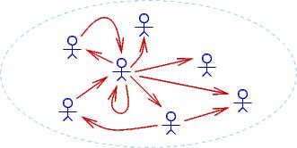
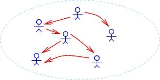
The examples of bosses and workers illustrate these points:-
You must state the domain of individuals when you state
premises. In the bosses-workers examples, the domain is
a collection of people. Both the bosses and the workers belong
to that domain. Here are three drawings of possible different domains,
where an arrow, person1 ---> person2, means that person1 is the
boss of person2:
Notice that FORALLuEXISTv isBossOf(v,u) (``everyone has a boss'') holds true for the first two domains but not the third. EXISTxFORALLy isBossOf(x,y) holds true for only the second domain.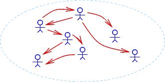
-
When we make a proof of P |- Q and P holds true for a domain,
then Q must also hold true for that same domain..
We proved that
EXISTxFORALLy isBossOf(x,y) |- EXISTz isBossOf(z,z),
and sure enough, in the second example domain,
EXISTz isBossOf(z,z) holds true.
Our logic system is designed to work in this way! When we do a logic proof, we are generating new facts that must hold true for any domain for which the premises hold true. This property is called soundness of the logic, and we will examine it more closely in a later section in this chapter.
-
A domain can have infinitely many individuals.
Here is a drawing of a domain of infinitely many people,
where each person bosses the person to their right:
In this domain, FORALLuEXISTv isBossOf(v,u) holds true as does FORALLuEXISTv isBossOf(u,v) (``everyone bosses someone''), but EXISTz isBossOf(z,z) does not hold true.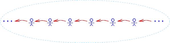
. . . < -3 < -2 < -1 < 0 < 1 < 2 < 3 < . . .Indeed, one of the main applications of logic is proving properties of numbers. This leads to a famous question: Is it possible to write a collection of premises from which we can deduce (make proofs of) all the logical properties that hold true for the domain of integers?
The answer is NO. In the 1920s, Kurt Goedel, a German PhD student, proved that the integers, along with +, -, *, /, are so complex that it is impossible to ever formulate a finite set (or even an algorithmically defined infinite set) of premises that generate all the true properties of the integers. Goedel's result, known as the First Incompleteness Theorem, set mathematics back on its heels and directly led to the formulation of theoretical computer science (of which this course is one small part). There is more material about Goedel's work at the end of this chapter.
Tactics for the EXIST-rules
There are two tactics; neither is easy to master:-
(***) EXISTe-tactic: To prove Premises, EXISTx Px |- Q,
- assume a and Pa, where a is a brand new anonymous name
- prove Premises, Pa |- Q
- apply EXISTe
1. Premises premise 2. EXISTx Px premise ... i. a ... Pa assumption (fill in) ... j. Q (does not mention a!) k. Q EXISTe 2,i-j -
(*) EXISTi-tactic: To prove Premises |- EXISTx Px,
try to prove Pe for some e that already appears in the partially
completed proof. Finish with EXISTi:
1.  Premises    premise
  . . .
i.  ...e...
      (fill in)
j.  Pe
k.  EXISTx Px  EXISTi j
6.2.1 Applications of the existential quantifier
Since an existential quantifier hides knowledge, it is useful to describe a function that returns some but not all the information that the function computes. Here is a simple example, for a computerized Wheel-of-Fortune game:===================================================
board = ... """{ invariant: isStringArray(board) ^ len(board) > 0 }"""
def gameOver() :
"""examines board to see if all squares uncovered. Returns True if so,
otherwise returns False."""
"""{ gameOverpre true }"""
"""{ gameOverpost answer --> ~(EXIST 0 <= i < len(board), board[i] == "covered")
^ ~answer --> (EXIST 0 <= i < len(board), board[i] == "covered")
}"""
answer = True
... while loop that searches board for a board[k] == "covered";
if it finds one, it resets answer = False ...
return answer
===================================================
The computerized Pat Sajak would use this function like this:
===================================================

done = gameOver()
if done :
    print "We have a winner!  Time for a commercial!"
else :
    print "There is still a letter that is covered. Let's continue!"

===================================================
Here is the relevant deduction:
===================================================

done = gameOver()
"""{  assert:  [done/answer]gameOverpost  }"""
if done :
    """{  1. done     premise
       2. [done/answer]gameOverpost   premise
       3. done --> ~(EXIST 0 < i < len(board), board[i] == "covered")   ^e 2
       4. ~(EXIST 0 < i < len(board), board[i] == "covered")  -->e 3,1 }"""
    print "We have a winner!  Time for a commercial!"
else :
    """{  1. ~done     premise
       2. [done/answer]gameOverpost   premise
       3. ~done --> (EXIST 0 < i < len(board), board[i] == "covered")   ^e 2
       4. EXIST 0 < i < len(board), board[i] == "covered"  -->e 3,1 }"""
    print "There is still a letter that is covered. Let's continue!"

===================================================
Notice that the answer returned by gameOver hides which square on the
board is still covered (== "covered").
We repeat an example from a previous chapter to show another use
of the existential:
===================================================

def delete(c, s) :
    """delete locates an occurrence of  c  in  s  and
       removes it and returns the resulting string.
       If  c  is not in  s, a copy of  s  is returned, unchanged.
    """
    """{  pre: isChar(c) ^ isString(s) }"""
    """{  post:  (EXIST 0 <= k < len(s), s[k] == c ^ answer == s[:k] + s[k+1:])
                v
              (FORALL 0 <= i < len(s), s[i] != c) ^ answer == s }"""
    index = 0
    found = False
    while index != len(s)  and  not found :
        """{  invariant (FORALL 0 <= i < index, s[i] != c)  ^
                              (found -->  s[index] == c)   }"""
        if  s[index] == c :
            found = True
        else :
            index = index + 1
    """{  assert: (index == len(s) v found)  ^  above invariant  }"""
    if found :
        answer = s[:index] + s[index+1:]
        """{  1. found                             premise
           2. answer == s[:index] + s[index+1:]  premise
           3. invariant                         premise
           4. (found -->  s[index] == c)    ^e 3
           5. s[index] == c                      -->e 4,1
           6. s[index] == c ^ answer == s[:index] + s[index+1:]  ^i 5,2
           7. 0 <= index < len(s)               algebra 5
           8. EXIST 0 <= k < len(s), s[k] == c ^ answer == s[:k] + s[k+1:]  EXISTi 7,6  (where [k/index])
       }"""
    else :
        answer = s
        """{  1. ~found                premise
           2. answer == s               premise
           3. (index == len(s) v found) premise
           4. invariant                premise
           5. index == len(s)           by  P v Q, ~Q |- P, 3,1
           6. FORALL 0 <= i < index, s[i] != c  ^e 4
           7. FORALL 0 <= i < len(s), s[i] != c   substitution 5,6
           8. (FORALL 0 <= i < len(s), s[i] != c) ^ answer == s  ^i 7,2
        }"""
    return answer

===================================================
The EXISTi rule is used inside the then-arm of the last conditional,
as shown above.
It is important that delete hide the value
of its local variable, index, from appearing in its postcondition,
because we do not want confusion like this:
===================================================

index = 2
t = "abcd"
u = delete("a", t)
"""{ at this point, we certainly cannot assert that t[2] = "a"! }"""

===================================================
6.2.2 The forwards assignment law uses an existential quantifier
The original, proper statement of the forwards assignment law reads like this:
"""{ assert: P }"""
x = e
"""{ assert: EXISTxold ( (x == [xold/x]e)  ^  [xold/x]P )  }"""
Our use of xold was hiding the quantifier.
Using EXIST, we can retain an assertion that uses the old value
of x.
In the earlier chapters, we worked examples like this:
===================================================

"""{ x > 0 }"""
x = x + 1
"""{ 1. xold > 0    premise
  2. x == xold + 1   premise
  3. x > 1          algebra 1,2
}"""

===================================================
and noted that xold must not appear in the last line of the proof.
The above proof is actually the subproof of a proof that finishes
with EXISTe! Here is the proper proof:
===================================================

"""{ x > 0 }"""
x = x + 1
"""{ 1. EXISTxold(xold > 0  ^  x == xold + 1)    premise
  ... 2. xold     xold > 0  ^  x == xold + 1      assumption
  ... 3. xold > 0                                        ^e1 2
  ... 4. x == xold + 1                                   ^e2 2
  ... 5. x > 1                                             algebra 3,4
  6. x > 1                    EXISTe 1, 2-5
}"""

===================================================
Again, it is crucial that xold not appear in the assertions on Lines
5 and 6.
We unconsciously use the existential quantifier and EXISTe every time we reason about the old, overwritten value of an updated variable.
Also,
when we introduce dummy names, like xin and
yin, to stand for specific values, as an example like this,
===================================================

"""{ assert: x == xin  ^  y == yin }"""
temp = x
x = y
y = temp
"""{ assert: x == yin  ^  y == xin }"""

===================================================
we are implicitly using existential quantifiers, again, like this:
===================================================

"""{ assert: EXISTxin EXISTyin(x == xin  ^  y == yin) }"""
temp = x
x = y
y = temp
"""{ assert: EXISTxinEXISTyin(x == yin  ^  y == xin) }"""

===================================================
6.3 The law for assigning to individual array elements
A key property of the forwards law for an assignment, x = e, is that the ``old'' value of x cannot appear in the final consequence that is deduced from the assignment. The same principle holds for assignment to an individual array element: a[e] = e' --- the ``old'' value of a[e] cannot appear in the assertion that results from the assignment.
For example,
if we have
"""{ assert: len(a) > 0 ^ FORALL 0 <= i < len(a), a[i] > 0 }"""
a[0] = 0
we should be able to deduce that
"""{ assert:  a[0] == 0
           ^  len(a) > 0
           ^  FORALL 0 < i < len(a), a[i] > 0
   implies:  FORALL 0 <= i < len(a), a[i] >= 0 }"""
How can we do this? The existing assignment law is too weak.
We require a special law for assignment to array elements.
The situation gets delicate if we are
unable to deduce the precise numerical value of the index
expression, e, in an assignment,
a[e] = e'.
Unless we can prove otherwise,
the assignment has essentially updated ``all'' of a!
Here is an example of a situation where we know nothing about
which cell was updated:
===================================================

n = readInt("Type an int between 0 and len(a)-1: ")
assert 0 <= n  and  n < len(a)
a[n] = a[n] - 1

===================================================
Clearly only one element of
a is decremented.
Let's try to reason about this situation:
===================================================

"""{ assert: FORALL 0 <= i < len(a), a[i] > 0 }"""

n = readInt("Type an int between 0 and len(a)-1: ")
assert 0 <= n  and  n < len(a)
"""{ assert: 0 <= n ^ n < len(a)  ^  FORALL 0 <= i < len(a), a[i] > 0 }"""

a[n] = a[n] - 1
"""{  assert:  a[n] == aold[n] - 1  ^  0 <= n  ^  n < len(a)
           ^  FORALL 0 <= i < len(a), aold[i] > 0
   implies: ???
}"""

===================================================
To move forwards, we must assert that all those variables a[i], such
that i != n, retain their old values:
===================================================

a[n] = a[n] - 1
"""{ 1. a[n] == aold[n] - 1                                 premise
  2. FORALL 0 <= i < len(a), (i!=n) --> a[i] == aold[i]   premise  NEW!
  3. 0 <= n ^ n < len(a)                             premise
  4. FORALL 0 <= i < len(a), aold[i] > 0                 premise
  5.  ...
}"""

===================================================
We accept the assertion (premise) on line 2 as a fact, and the forwards assignment law
for arrays includes this fact ``for free'' as part of its postcondition.
Here is the law for array assignment:
"""{ assert: P }"""
a[e] = e'    # where  e  contains _no mention_ of  a
"""{ 1. a[e] == e'        premise
  2. [aold/a]P                      premise
  3. FORALL 0 <= i < len(a), (i != e) --> a[i] == aold[i]   premise
  4. len(a) == len(aold)            premise
     ...
  n. Q    # must not mention aold
}"""
We gain the new premises in lines 3 and 4. Line 2 is used
with FORALLe
to extract information about array elements that
were not affected by the assignment to a[e].
Now we have enough knowledge to make a useful deduction:
===================================================

a[n] = a[n] - 1
"""{ 1. a[n] == aold[n] - 1                                        premise
  2. FORALL 0 <= i < len(a), (i!=n) --> a[i] == aold[i]  premise
  3. 0 <= n ^ n < len(a)                                    premise
  4. FORALL 0 <= i < len(a), aold[i] > 0                      premise
  5. aold[n] > 0                                               FORALLe 4,3
  6. a[n] >= 0                                                   algebra 1,5
           (next, we salvage the facts about those  a[i] such that i != n: )
  ... 8.  0 <= x < len(a)                    assumption
  ... 9.  aold[x] > 0                      FORALLe 4,8
  ... 10. (x!=n) --> a[x] == aold[x]   FORALLe 2,8
  ... ... 11. x != n                            assumption
  ... ... 12. a[x] == aold[x]                  -->e 10,11
  ... ... 13. a[x] > 0                          algebra 9,12
  ... 14. (x!=n) --> a[x] > 0          -->i 11-13
  15. FORALL 0 <= x < len(a): (x!=n) --> a[x] > 0  FORALLi 8-14

  16. a[n] >= 0 ^ FORALL 0 <= x < len(a): (x!=n) --> a[x] > 0  ^i 6,15  }"""

===================================================
This tedious proof shows the difficulty in reasoning precisely about
an array update with an unknown index value.
It is easy to be discouraged by the length of the
above proof, which says that the nth element of
a was changed.
For this reason, some researchers use a picture notation to encode
the assertions.
For example, the assertion,
FORALL 0 <= i < len(a), a[i] > 0
Might be drawn like this:
      0  1  ... len(a)-1
    +--+--+-- --+--+
a = |>0|>0| ... |>0|
    +--+--+-- --+--+
so that after the assignment, a[n] = a[n]-1, we deduce this
new pictorial assertion:
      0  1 ...    n  ...  len(a)-1
    +--+--+-   -+---+    -+--+
a = |>0|>0| ... |>=0| ... |>0|
    +--+--+-   -+---+    -+--+
which is meant to portray
a[n] >= 0 ^ FORALL 0 <= x < len(a), (x!=n) --> a[x] > 0.
These pictures can be helpful for informal reasoning, but they quickly get confusing. (For example, where do you draw n's cell in the above picture? What if n == 0? Etc.) Use such drawings with caution.
To summarize, the forwards assignment law for individual
array elements reads as follows:
"""{ assert: P }"""
a[e] = e'    # where  e  contains _no mention_ of  a
"""{ assert:  a[e] == e'
           ^  FORALL 0 <= i < len(a), (i != e) --> a[i] == aold[i]
           ^  len(a) == len(aold)
           ^  [aold/a]P
}"""
6.4 Case studies
6.4.1 In-place selection sort
When an array holds elements that can be ordered by <, it is useful to rearrange the elements so that they are ordered (sorted). There are several useful tecniques to sort an array's elements in place, that is, move them around within the array until the array is sorted.One useful and straightforward technique is selection sort, where the unsorted segment of the array is repeatedly scanned for the smallest element therein, which is extracted at moved to the end of the array's sorted segment.
A trace of a selection sort would look like this:
===================================================

  (sorted segment) | (unsorted segment)
                   v
              a == ["f", "d", "c", "b", "e"]
                   v
          a == ["b", "d", "c", "f", "e"]   ("b" selected and moved to front
                   v                            by exchanging it with "f")
     a == ["b", "c", "d", "f", "e",]   ("c" selected and moved to front
                   v                        by exchanging it with "d")
a == ["b", "c", "d", "f", "e"]   ("d" selected and moved to front
                                      by exchanging it with itself)
(etc.)                       |
                             v
a ==  ["b", "c", "d", "e", "f"]   (finished)

===================================================
We require a function that searches the unsorted segment of the
array and locates the position of the least element therein:
===================================================

a = ["e", "d", "a", "c", "b" , "a"]   # data structure managed by this module

def select(start) :
   """select returns the index of the smallest element in array  a's
      segment from  a[start]...a[len(a)-1]."""
   """{ pre:  0 <= start < len(a)  }"""
   """{ post: start <= answer < len(a)  ^
            FORALL start <= i < len(a), a[answer] <= a[i]  }"""
   answer = start
   index = start + 1
   """{ invariant:  FORALL start <= i < index, a[answer] <= a[i] }"""
   while index != len(a) :
       if  a[index] < a[answer] :
          answer = index
       index = index + 1
   return answer

===================================================
The pre-postconditions tell us
the knowledge the function computes.
Next, define these notions of ``ordered'' and ``permuted'' for arrays:
ordered(a) =  FORALL 0 < i < len(a), a[i-1] <= a[i]
perm(a, b) =  (len(a) = len(b))  ^  (elements of  a  ==  elements of b)
The second predicate states what it means for one array, a, to
have the same elements as another, b, but maybe in a different order.
It is a little informal but good enough for us to use here.
The function that does a selection sort uses a loop to repeatedly call select to find the elements to move to the front of the array.
Here's the function and the sketch of the proof. The loop invariant is key ---
the elements that have been already selected are moved
to the front of a are all guaranteed to be less-than-or-equal-to the elements
in a's rear that have not yet been selected:
===================================================

def selectionSort() :
   """does an in-place sort on global array  a,  using  select."""
   """{ pre  true
     post   ordered(a)  ^  perm(ain, a)   (Recall: ain is the starting value for  a) }"""
   global a

   index = 0
   """{ invariant   ordered(a[:index])  ^  perm(a, ain)  ^
                 FORALL 0 <= i < index, FORALL index <= j < len(a), a[i] <= a[j] }"""
   while index != len(a) :
      x = select(index)
      """{ assert: start <= x < len(a)  ^
                 FORALL index <= i < len(a), a[x] <= a[i]
                 ^  invariant  }"""
      least = a[x]       # exchange the least element with the one at the
      a[x] = a[index]    #  front of the unsorted segment
      a[index] = least
      """{  assert: ordered(a[:index])  ^  perm(a, ain) ^
                 index <= x < len(a) ^
                 a[index] = least  ^
                 FORALL index < i < len(a), least <= a[i]
        implies: FORALL 0 <= i < index, a[i] <= least
        implies: ordered(a[:index+1])  ^
                 FORALL 0 <= i < index+1, FORALL index+1 <= j < len(a): a[i] <= a[j] }"""
      index = index + 1
      """{  assert: invariant }"""

===================================================
The
key accomplishment of
least = a[x]
a[x] = a[index]
a[index] = least
is to move the least element in the unsorted suffix of a to
the front of that suffix. But that makes the least value eligible
to be the rear element of the sorted prefix of a.
In this way, the loop's invariant is restored as we finish with
index = index + 1.
6.4.2 Binary search
Once an array is sorted, it can be searched for a value quickly, much like you search for a word in a dictionary: you open the dictionary in the middle and see if you got lucky and found the word. If so, you are finished. If the word is earlier in the dictionary, then you ignore the back half of the book and instead split open the front half. (And vice versa for a word located in the back half in the dictionary.) You repeat this technique till you find the page where your word is.We can search a sorted array, a, for a value, v, but jumping in the middle of a. If we find v there, we are done. Otherwise, we repeat the step, jumping into the first half or the second half, as needed. Eventually, we find the value (if it is there).
Here is the function, which is famous for its difficulty to
write correctly. Glance at it, then read the paragraph
underneath it, then return to the function and study its assertions:
===================================================

def search(v, lower, upper) :
   """searches for value  v  within array  a  in the range  a[lower]...a[upper].
      If found, returns the index where  v  is; if not found, returns -1"""
   """{  searchpre   ordered(a)  ^
            FORALL 0 <= i < lower, a[i] < v  ^
            FORALL upper < j < len(a): v < a[j]
                (That is,  v  isn't in  a[:lower]  and  a[upper+1:].)  }"""
   """{  searchpost   ((0 <= answer < len(a))  ^  a[answer] == v)  v
                     (answer = -1  ^  FORALL 0 <= i < len(a), v != a[i]) }"""

   if  upper < 0  or  lower > len(a)-1  or  lower > upper :  # empty range to search?
      """{  assert: (upper < 0  v  lower > len(a)-1  v  lower > upper)  ^
                 searchpre
         implies:  FORALL 0 <= i < len(a), v != a[i] }"""
      answer = -1
      """{  assert:  answer = -1  ^  (FORALL 0 <= i < len(a), v != a[i]),
                  that is,  searchpost  }"""
   else :
      index = (lower + upper) / 2
      if  v == a[index] :  # found v at a[index] ?
         answer = index
         """{  assert: a[answer] == v
            implies: searchpost }"""
      elif  v > a[index] :
         """{  assert: v > a[index]  ^  searchpre
            implies: FORALL 0 <= i <= index, a[i] < v
            implies: [index+1/lower]searchpre  }"""
         answer = searchFor(v, index+1, upper)
         """{  assert:  searchpost  }"""
      else :  # a[index] < v
         """{  assert: a[index] < v  ^  searchpre
            implies:  FORALL index <= j < len(a), v < a[j]
            implies:  [index-1/upper]searchpre  }"""
         answer = searchFor(v, lower, index-1)
         """{  assert:  searchpost  }"""
   """{  assert: searchpost  }"""
   return answer

===================================================
To search array, a, for v, we start the function like this:
search(v, 0, len(a)-1)
The precondition is the key: to use correctly
search(v, lower, upper), we must already know that v is
not in a[0]...a[lower-1] and not in
a[upper+1}...a[len(a)-1] --- we have already narrowed the search
to the range of a[lower]...a[upper].
The function builds on this fact to narrow further the search in subsequent
self-calls until v is found or there is an empty range left to search.
The previous two examples display a style of documentation that is used when correctness is critical and one is unable to perform enough testing to generate high confidence that the coding is correctly --- the program must be correct from the first time is it used. Such an approach is taken with safety-critical systems, where money and life depend on the correct functioning of software from the moment it is installed.
6.4.3 Maintaining a board game: programming by contract
Many programs maintain a data structure like an edit buffer or a spreadsheet or a game board. Typically, the data structure is grouped with its maintenance functions (in its own module or class). This is often called the model component, because the data structure is a computerized ``model'' of a real-life object. Next, there is a controller component (module/class) that interacts with the user and calls the maintenance functions in the model component. (The controller sets the protocol and ``controls'' and ``connects'' the interactions between user and model.) If there is a graphical user interface to paint and maintain, yet another component, called the view, must be written. This trio of components forms a standard software architecture, called the model-view-controller architecture.To build such a system, we must document the internal structure and connection points of each component so that the system can be connected correctly. This documentation is exactly the pre- and post-conditions for the functions in each component as well as the invariants for the data structures therein.
Here is a small example. It is an implementation of a tic-tac-toe game that follows the usual rules.
First, there is the model module, which models the game board as
an array.
The game board has an important invariant
that ensures that only legal game tokens are placed on the board.
There is another data structure in this module that remembers the history of
moves made on the board.
Both data structures are documented with their invariants.
(If you are programming in an object-oriented language and have
written a class to model the game board, you call the data-structure
invariants, class invariants.
===================================================

"""module GameBoard  models a Tic-Tac-Toe board.

   There are two key data structures:
   --- board,  the game board, which holds the players' moves
   --- history,  a list of all the moves made during the game

   The data structures are managed by calling the functions defined
   in this module.
"""

# The game players:
X = "X"
O = "O"
NOBODY = "neither player"

###### The game board, a matrix sized  dimension x dimension:
EMPTY = "_"     # marks an empty square on the board
dimension = 3
BOARDSIZE = dimension * dimension
# the board itself:
board = []    # construct the board with this loop:
i = 0
while i != dimension :
    board.append(dimension * [EMPTY])
    i = i + 1
"""{ global invariant for board:  Only legal markers are placed on it
      ALL 0 < i,j < dimension,
          board[i][j] == X  v  board[i][j] == O  v  board[i][j] == EMPTY }"""

#### A history log of all the moves:  it is a list of  Marker, Row, Col  tuples:
history = []
"""{ global invariant for history:  All moves in  history  recorded in  board
      forall 0 < i < len(history), history[i]==(m,r,c)  and  board[r,c] == m
}"""

### Functions that manage the  board  and  history:

def printBoard() :
    """prints the board on the display"""
    """{  pre   true
          post  forall 0 <= i,j < dimension, board[i][j] is printed  }"""
    counter = 0
    for row in board :
        for square in row :
            if square != EMPTY :
                print square,
            else :
                print counter,
            counter = counter + 1
        print
    print
    #print history


def emptyAt(position) :
    """examines the ith square on board;  returns whether it equals EMPTY.

       params: position - an int that falls between 0 and the BOARDSIZE
       returns: whether or not square number  position on  board  is EMPTY
    """
    """{ pre   0 <= position < BOARDSIZE
        post  answer == (board[position/dimension][position%dimension] == EMPTY) }"""
    answer = False
    (row,col) = (position/dimension, position%dimension)
    if  0 <= row  and  row < dimension  and  0 <= col  and  col < dimension \
       and  board[row][col] == EMPTY :
        answer = True
    return answer


def move(marker, position) :
    """attempts to move  marker  into the board at  position

       params: marker - a string, should be  X  or  O
               position -- an int, should be between 0 and the BOARDSIZE
    """
    """{  pre  ((marker == X) v (marker == O)) &  (0 <= position < BOARDSIZE)
          post   invariants for board and history are maintained }"""
    global history, board   # because we update these global variabes,
                            # we are OBLIGATED to maintain their invariants!
    if emptyAt(position) :
        (row,col) = (position/dimension, position%dimension)
        board[row][col] = marker
        history = history + [(marker,row,col)]
    else :
       pass

def winnerIs(mark) :
    """checks the game board to see if  mark  is the winner.

       parameter:  mark - a string, should be  X  or  O
       returns:  mark,  if it fills a complete row, column, or diagonal of
                 the board;  returns  NOBODY, otherwise.
    """
    """{  pre  (mark == X) v (mark == O)
          post: (answer == mark -->  mark has filled a row or column or diagonal)
              and  (answer == NOBODY) --> mark has not filled any row/col/diag}"""

    def winnerAlong(vector) :
        """sees if all the elements in  vector  are filled by  mark"""
        check = True
        for index in range(dimension):
            check = check and (vector[index] == mark)
        return check

    # check  row i  and  column i  for  i in 0,1,...,dimension-1:
    for i in range(dimension) :
        columni = []
        for j in range(dimension):
            columni = columni + [board[j][i]]
        if winnerAlong(board[i]) or winnerAlong(columni) :
            return mark

    # check the left and right diagonals:
    ldiag = []
    rdiag = []
    for i in range(dimension):
        ldiag = ldiag + [board[i][i]]
        rdiag = rdiag + [board[i][(dimension-1)-i]]
    if winnerAlong(ldiag) or winnerAlong(rdiag) :
        return mark
    # else, no winner, so
    return NOBODY

===================================================
The data-structure invariants establish the internal well-formedness of
the game board, and the maintenance functions are obligated
to preserve and maintain
the invariants.
In addition, each function is documented with its own pre-post conditions
that specify how the function should be called and what the function
guarantees if it is called correctly. In the above coding, both
informal English and formal logical specifications are written.
Whether one writes English or logic depends on how critical
absolute correctness might be. (Frankly, some programs, e.g.,
toys and games, need not be absolutely correct.)
The other module of this little example is the main program --- the controller module --- which enforces the rules of the game, that is, the proper interaction of the game's players with the game board. The controller's main loop has its own invariant that asserts this point. The loop
- displays the game board
- requests a player's next move
- implements the move on the board
===================================================

"""The Main module controls the tic-tac-toe game."""

import GameBoard
from GameBoard import *

def readInt(message):
    """readInt is a helper function that reads an int from the display.
       If we had a View Module that painted a GUI, this function would
       be found there.

       param: message a string
       returns: an int, denoting the number typed by a player
    """
    """{  pre:  message:String
          post: answer:int  }"""
    needInput = True
    answer = ""
    while needInput :
        text = raw_input(message)
        if text.isdigit() :
            answer = int(text)
            needInput = False
    return answer

player = X       # whose turn is it?  who goes first?
count = 0        # how many moves have been made?
winner = NOBODY  # who is the winner?

"""{  loop invariant:  The rules of the tic-tac-toe game are enforced:
      (i) players take turns moving:
            forall 0 <= i < count,
               (i % 2)== 0 -->  history[i][0] == X   and
               (i % 2)== 1 -->  history[i][0] = O
      (ii) all moves are recorded on board:
             invariant for  history  remains true;
      (iii) board holds only legal game markers:
             invariant for  board  remains true
        (NOTE: (ii) and (iii) should hold automatically provided
        that we use the board's maintenance functions.)
}"""
while winner == NOBODY  and  count != BOARDSIZE :

    printBoard()

    # get the next move:
    awaitingMove = True
    while awaitingMove :
        """{ invariant
                  awaitingMove --> (0 <= m < BOARDSIZE) and emptyAt(m) }"""
        m = readInt("Player " + player +  \
                    ": type next move (0.." + str(BOARDSIZE) + "): ")

        if (0 <= m) and (m < BOARDSIZE) and emptyAt(m) :
            awaitingMove = False

    # we have received a legal move:
    """{ assert: ((player == X) v (player == O))
                   and (0 <= m < BOARDSIZE) and  emptyAt(m)
         implies:  [player/marker][m/position]movepre  }"""
    move(player, m)
    """{  assert:  movepost, that is,
          invariants for  board  and   history  are maintained }"""

    # determine whether this player is the winner:
    winner = winnerIs(player)

    # switch players for the next round:
    if player == X :
        player = O
    else :
        player = X
    count = count + 1

    """{ assert: loop invariant, all 3 parts, holds }"""

# the loop quit, and the game's over:
print winner + " won!"
printBoard()

===================================================
Note how the controller uses the pre-post-conditions for the board's
maintenance functions to fulfill its own invariants.
In this way, we depend on the documentation from one module to
program correctly another. Programming in this style is sometimes
called programming by contract.
6.4.4 Maintaining a spelling tree
To come.6.5 Equivalences in predicate logic
Here are some important equivalences in predicate logic:- FORALLx FORALLy Pxy -||- FORALLy FORALLx Pxy
- EXISTx EXISTy Pxy -||- EXISTy EXISTx Pxy
- ~(FORALLx Px) -||- EXISTx ~Px
- ~(EXISTx Px) -||- FORALLx ~Px
- Q ^ (FORALLx Px) -||- FORALLx (Q ^ Px) (where x does not appear in Q)
- Q v (FORALLx Px) -||- FORALLx (Q v Px) (where x does not appear in Q)
- Q ^ (EXISTx Px) -||- EXISTx (Q ^ Px) (where x does not appear in Q)
- Q v (EXISTx Px) -||- EXISTx (Q v Px) (where x does not appear in Q)
6.6 Predicate logic without the existential quantifier: Skolem functions
Complexity arises in predicate logic when a proposition contains a mix of FORALL and EXIST. Recall that FORALLx EXISTy P(x,y) asserts that each element named by x ``has its own personal'' y to make P(x,y) true. (``Everyone has a boss.'') In contrast, EXISTy FORALLx P(x,y) identifies one single individual that is related to all elements, x, to make P(x,y) true. (``There is one boss who is the boss of everyone.'')
Logicians have developed a form of predicate logic that omits the
existential quantifier and uses instead terms called Skolem
functions to name the values represented by each EXISTy.
A Skolem function is a function name
that is used to designate where an existential quantifier should appear.
Examples explain the idea best:
===================================================

Everyone has a boss:                     FORALLx EXISTy P(x,y)
(expressed with a Skolem function,
  named  boss:)                          FORALLx P(x, boss(x))

There is a single boss of everyone:      EXISTy FORALLx P(x,y)
(expressed with a Skolem function,
  named  bigb:)                          FORALLx P(x, bigb())

For every husband and wife, there
is a minister who married them:          FORALLx FORALLy EXISTz M(z,x,y)
(expressed with a Skolem function,
named minister:)                         FORALLx FORALLy M(minister(x,y),x,y)

Every two ints can be added into
a sum:                                   FORALLx FORALLy EXISTz F(x,y,z)
(expressed with a Skolem function,
named sum:)                              FORALLx FORALLy F(x,y,sum(x,y))

Every boss has a secretary,
who talks with everyone:                 FORALLx EXISTy (isSec(y) ^ FORALLz talks(x,z))
(expressed with a Skolem function,
named  s:)                               FORALLx (isSec(s(x)) ^ FORALLz talks(s(x),z))

===================================================
The examples show how the Skolem function acts as a ``witness'' to the
missing EXIST without revealing the identity of the individual discussed.
You can also see the difference in the first two examples between
boss(x) and bigb() --- the first example makes clear how the boss is
a function of which x in the domain is considered; the second one
makes clear that the boss is independent of all the individuals in the domain.
It is possible to work proofs in predicate logic with
Skolem functions. Here are two examples:
===================================================

FORALLx isMortal(x) --> hasSoul(x),  isMortal(socrates()) |- hasSoul(t())

1. FORALLx isMortal(x) --> hasSoul(x)                    premise
2. isMortal(socrates())                            premise
3. isMortal(socrates()) --> hasSoul(socrates())     FORALLe 1
4. hasSoul(socrates())                             -->e 3,2
6. hasSoul(t())                                    def t(): return socrates()

===================================================
Here, the individual, Socrates, is represented as a constant
Skolem function, socrates().
The key step is the last one, where the desired Skolem function,
t(), is defined in terms of socrates():
def t() :
    return socrates()
This function definition takes the
place of EXISTi.
In the previous example, we could have read isMortal(socrates()) as a shorthand for EXISTsocrates (isMortal(socrates)). Now, there is no practical difference.
Here is the boss-worker example (``if someone is the boss of everyone,
then everyone has a boss''):
===================================================

FORALLx isBossOf(x, big()) |- FORALLx isBossOf(x, b(x))

1. FORALLx isBossOf(x, big())     premise
... 2. a
... 3. isBossOf(a, big())        FORALLe 1
... 4. hasBoss(a, b(a))          def b(a): return big()
5. FORALLx is BossOf(x, b(x))     FORALLi 2-4

===================================================
Notice how the defined Skolem function, b(a), disregards its
argument and always returns big() as its answer. This is because
big() is truly a's boss, no matter what argument is assigned
to parameter a.
Like before, it is impossible to prove FORALLx isBossOf(x, b(x)) |- FORALLx isBossOf(x, big()) --- there is no way to define a Skolem function, def big() : ... b(x) ..., because a value for parameter x is required. In this way, the Skolem functions ``remember'' the placement and use of the original existential quantifiers.
The technical reasoning why Skolem functions work correctly requires so-called Herbrand models and the Henkin completeness theorem. But the programming intuition given here --- defining Skolem functions as Python functions --- works surprisingly well.
6.7 Resolution theorem proving for predicate logic
Skolem functions make it possible to adapt the resolution-theorem-proving technique from the previous chapter to predicate logic. The key idea is to convert all propositions into and-or form, remove the existential quantifers, then move and remove the universal quantifiers (!), then complete the transformation into conjunctive-normal form. Then, we can perform resolution theorem proving with the aid of unification (two-way matching) of Skolem functions.Conversion into clause form
Conjunctive-normal form for predicate calculus is called clause form. We achieve clause form in these steps:- First, rename as needed all variables, x, used within all quantifiers, FORALLx and EXISTx, so that each occurrence of a quantifier appears with a unique variable name.
-
Remove all implications, A --> B, with this
equivalence:
A --> B -||- ~A v B
-
Next, move all remaining negation operators inwards, by repeatedly
applying these equivalences:
~(A ^ B)  -||-  ~A v ~B
~(A v B)  -||-  ~A ^ ~B
~(FORALLx A) -||- EXISTx ~A
~(EXISTx A) -||- FORALLx ~A
and wherever it appears, replace ~~A by A. - Remove all existential quantifiers, replacing their variables by Skolem functions.
-
Use these equivalences to move all occurrences of
universal quantifiers to the leftmost position of the proposition:
Q ^ (FORALLx Px) -||- FORALLx (Q ^ Px)
Q v (FORALLx Px) -||- FORALLx (Q v Px)
(This is called prenex form.) Now, remove the quantifiers because they are no longer needed (!). -
At this point, all quantifiers are removed, and the proposition
is a combination of conjunctions, disjunctions, and negations attached
to primitive propositions that hold Skolem functions.
To finish, apply this equivalence to
move all disjunction operators inward:
(A ^ B) v C -||- (A v C) ^ (B v C)
===================================================

1. (EXISTy FORALLx isBossOf(y,x)) --> (EXISTz isBossOf(z,z))

2. ~(EXISTy FORALLx isBossOf(y,x))  v (EXISTz isBossOf(z,z))

3. (FORALLy ~FORALLx isBossOf(y,x))  v (EXISTz isBossOf(z,z))
   (FORALLy EXISTx ~isBossOf(y,x))  v (EXISTz isBossOf(z,z))

4. (FORALLy ~isBossOf(y, x(y))   v  isBossOf(z(),z())

5. FORALLy ( ~isBossOf(y, x(y))   v  isBossOf(z(),z()) )

   (~isBossOf(y, x(y)))  v  isBossOf(z(),z())

6. (no need to rearrange any ^s and vs)

===================================================
At this point, we can apply the resolution algorithm. The resolution rule is slightly modified to handle the variables and Skolem functions: a form of two-way matching, called unification, is used to apply the FORALLe rule to variables and Skolem functions:
        A v P(E1)    ~P(E2) v B    matches = unify(E1,E2)
res:  ---------------------------------------------------------
             [matches](A v B)
Since P is now a predicate (like isBossOf or isMortal or >),
we must unify the arguments E1 and E2 in P(E1) and P(E2) so
that they become one and the same.
It works like this:
For example,
===================================================

for  isMortal(soc())   ~isMortal(z),      unify(soc(),z) =  [z=soc()]

for  isMortal(x)       ~isMortal(y),      unify(x,y) = [x=y]

for  isBoss(a(),x)     ~isBoss(y,b()),    unify((a(),x), (y,b())) = [y=a(), x=b()]

for  isBoss(a(),x)     ~isBoss(b(),b()),  unify((a(),x), (b(),b())) = FAILURE

===================================================
The matches that are computed are applied to the remaining clauses. For example,
~P(x) v Q(x)        P(a())
-------------------------------
             Q(a())
because matches(x,a()) = [x=a()], so [x=a()]Q(x) is Q(a()).
We apply the revised resolution rule to proving contradictions, like we did with propositional logic. The resolution rule plus unification searches for a witness to a contradiction.
Here are two examples of resolution proofs conducted with unification:
===================================================

FORALLx (P(x) --> Q(x)),  EXISTy P(y)  |-  EXISTz Q(z)

The clauses resulting from the two premises and negated goal are
   ~P(x) v Q(x),   P(y()),   ~Q(z)

The resolution proof goes

~P(x) v Q(x)    P(y())    ~Q(z)
      |              |         |
      +--------------+         |
            | [x=y()]          |
           Q(y())              |
            |                  |
            +------------------+
                    | [z=y()]
                   []

===================================================
Here is another example, the workers-and-bosses proof:
===================================================

EXISTy FORALLx isBossOf(y,x)  |-  FORALLu EXISTv isBossOf(v,u)

      isBossOf(y(),x)              ~isBossOf(v, u())
           |                        |
           +------------------------+
                      | [v=y(), x=u()]
                     []

===================================================
Because a clause can be used more than once in a proof,
and because a variable can be set to a new value each time
it is unified in a resolution step, there is no guarantee that
the algorithm will always terminate with success or failure.
This is not a flaw of the algorithm --- predicate logic is
incomplete in that there can be no algorithm that can
decide whether or not a sequent can be proved.
Resolution is about as good as we can do in this regard.
6.8 Soundness and completeness of deduction rules
Once again, it is time to consider what propositions mean and how it is that FORALLi, FORALLe, EXISTi, EXISTe preserve meaning.At this point, it would be good to review the section on models for propositional logic in Chapter 5. There, we saw that the connectives, ^, v, ~, --> were understood in terms of truth tables. Also, the primitive propositions were just letters like P, Q, and R, which were interpreted as either True or False.
Within predicate logic, we use predicates, like isMortal() and >, to build propsitions, and we might also use functions, like +, within the predicates. We must give meanings to all predicates and functions so that we can decide whether propositions like isMortal(God) and (3+1)>x are True or False. The act of giving meanings to the predicates and functions is called an interpretation.
Interpretations
When we write propositions in a logic, we use predicates and function symbols (e.g., FORALLi (i*2)>i). An interpretation gives the meaning of- the underlying domain --- what set of elements it names;
- each function symbol --- what answers it computes from its arguments from the domain; and
- each predicate --- which combinations of arguments from the domain lead to True answers and False answers.
Here is an example. Say we have the function symbols, +,-,*,/, and predicate symbols, >,=. What do these names and symbols mean? We must interpret them
-
The standard interpretation of arithmetic is that
int
names the set of all integers; +,-,*,/ name
integer addition, subtraction, multiplication, and division, and
= and > name integer equality comparison
and integer less-than comparison.
With this interpretation of arithmetic, we can interpret propositions.
For example, FORALLi (i*2)>i interprets to False,
and EXISTj (j*j)=j interprets to True.
If we use any extra, ``constant names,'' (e.g., pi), we must give
meanings to the constants, also.
-
Now, given function names +,-,*,/,
and predicates, =, >, we can choose to interpret them in another
way. For example, we might interpret the underlying domain as just
the nonnegative integers. We can interpret +,*,/,>,= as the usual
operations on ints, but we must give a different meaning to -.
We might define m - n == 0, whenever n > m.
- Yet another interpretation is to say that the domain is just {0,1}; the functions are the usual arithmetic operations on 0,1, modulo 2; and > is defined 1 > 0 (and that's it).
These three examples show that the symbols in a logic can be interpreted in multiple different ways. (In Chapter 5, we called an interpretation a ``context.'' In this chapter, we see that a ``context'' is quite complex --- domain, functions, and predicates.)
Here is a second example. There are no functions, and the predicates are isMortal(_), isLeftHanded(_), isMarriedTo(_,_). An interpretation might make all (living) members of the human race as the domain; make isMortal(h) True for every human, h; make isLeftHanded(j) True for exactly those humans, j, who are left handed; and set isMarriedTo(m,f) True for all pairs of humans m, f, who have their marriage document in hand.
You get the idea....
We can ask whether a proposition is True within one specific interpretation, and we can ask whether a proposition is True within all possible interpretations. This leads to the notions of soundness and completeness for predicate logic:
A sequent, P1, P2, ..., Pn |- Q is valid in an interpretation, I, provided that when all of P1, P2, ..., Pn are True in interpretation I, so is Q. The sequent is valid exactly when it is valid in all possible interpretations. We have these results for the rules of propositional logic plus FORALLi, FORALLe, EXISTi, EXISTe:
- soundness: When we use the deduction rules to prove that P1, P2, ..., Pn |- Q, then the sequent is valid (in all possible interpretations).
- completeness: When P1, P2, ..., Pn |- Q is valid (in all possible interpretations), then we can use the deduction rules to prove the sequent.
In the early 20th century, Kurt Gödel showed that it is impossible to formulate a sound set of rules customized for arithmetic that will prove exactly the True facts of arithmetic. Gödel showed this by formulating True propositions in arithmetic notation that talked about the computational power of the proof rules themselves, making it impossible for the proof rules to reason completely about themselves. The form of proposition he coded in logic+arithmetic stated ``I cannot be proved.'' If this proposition is False, it means the proposition can be proved. But this would make the rule set unsound, because it proved a False claim. The only possibility is that the proposition is True (and it cannot be proved). Hence, the proof rules remain sound but are incomplete.
Gödel's construction, called diagonalization, opened the door to the modern theory of computer science, called computability theory, where techniques from logic are used to analyze computer programs. Computability theory tells us what problems computers cannot solve, and why, and so we shouldn't try. (For example, it is impossible to build a program-termination checker that works on all programs --- the checker won't work on itself!) There is also an offshoot of computability theory, called computational complexity theory, that studies what can be solved and how fast an algorithm can solve it.
Given an interpretation of a predicate logic, we can say that the ``meaning'' of a proposition is exactly the set of interpretations (cf. Chapter 5 --- ``contexts'') in which the proposition is True. This returns us to the Boolean-algebra model of logic in Chapter 5. Or, we can organize the interpretations so that an interpretation grows in its domain and knowledge over time. This returns us to the Kripke models of Chapter 5. Or, we can introduce two new programming constructs, the abstract data type and the parametric polymorphic function and extend the Heyting interpretation in Chapter 5.
All of these are possible and are studied in a typical second course on logic.
6.9 Summary
Here are the rules for the quantifiers, stated in terms of their tactics:-
(***) FORALLi: use to prove Premises |- FORALLx Px:
1. Premises premise ... i. a (fill in) ... j. Pa k. FORALLx Px FORALLi i-j -
(*) FORALLe-tactic: use to prove Premises, FORALLx Px |- Q,
1. Premises premise 2. FORALLx Px premise . . . j. Pa FORALLe j (fill in) k. Q -
(**) EXISTe-tactic: use to prove Premises, EXISTx Px |- Q:
1. Premises premise 2. EXISTx Px premise ... i. a ... Pa assumption (fill in) ... j. Q (does not mention a!) k. Q EXISTe 2,i-j -
(*) EXISTi-tactic: use to prove Premises |- EXISTx Px:
1.  Premises    premise
  . . .
i.  ...e...
      (fill in)
j.  Pe
k.  EXISTx Px  EXISTi j